Foreword
Following my last post on the “…first, second, and third dimensions, and why fractals don’t belong to any of them…“, this post is about documenting my journey as I delve deeper into the subject of fractals, mathematics, and geometry.
The study of fractals is an intensely vast topic. So much so that I’m convinced you could easily spend several lifetimes studying them. That being said, I chose to focus specifically on single-curve geometry. But, keep in mind that I’m only really scratching the surface of what there is to explore.
4.0 Classic Space-Filling
Inspired by Georg Cantor’s research on infinity near the end of the 19th century, mathematicians were interested in finding a mapping of a one-dimensional line into two-dimensional space – a curve that will pass through through every single point in a given space.
Jeffrey Ventrella writes that “a space-filling curve can be described as a continuous mapping from a lower-dimensional space into a higher-dimensional space.” In other words, an initial one-dimensional curve is developed to increase its length and curvature – the amount of space in occupies in two dimensions. And in the mathematical world, where a curve technically has no thickness and space is infinitely vast, this can be done indefinitely.
4.1 Early Examples
In 1890, Giuseppe Peano discovered the first of what would be called space-filing curves:

An initial ‘curve’ is drawn, then each element of the curve is replace by the whole thing. Here it is done four times, and it’s easy to imagine how you can keep doing this over and over again. One would think that if you kept doing this indefinitely, this one-dimensional curve would eventually fill all of two-dimensional space and become a surface. However it can’t, since it technically has no thickness. So it will be as close as you can get to a surface, without actually being a surface (I think.. I’m not that sure..)
A year later, David Hilbert followed with his slightly simpler space-filing curve:

In 1904, Helge von Koch describes a single complex continuous curve, generated with rudimentary geometry.

Around 1967, NASA physicists John Heighway, Bruce Banks, and William Harter discovered what is now commonly known as the Dragon Curve.

4.2 Later Examples
You may have noticed that some of these curves are better at filling space than others, and this is related to their dimensional measure. They fall under the category of fractals because they’re neither one-dimensional, nor two-dimensional, but sit somewhere in between. For these examples, their dimension is often defined by exactly how much space they fill when iterated infinitely.
While these are some of the earliest space-filling curves to be discovered, they are just a handful of the likely endless different variations that are possible. Jeffrey Ventrella spent over twenty-five years exploring fractal curves, and has illustrated over 200 hundred of them in his book ‘Brain-Filling Curves, A Fractal Bestiary.’ They are organised according to a taxonomy of fractal curve families, and are shown with a unique genetic code.
Incidentally, in an attempt to recreate one of the fractals I found in Jeffery Ventrella’s book, I accidentally created a slightly different fractal. As far as I’m concerned, I’ve created a new fractal and am unofficially naming it ‘Nicolino’s Quatrefoil.’ The following was created in Rhino and Grasshopper, in conjunction Anemone.

You can find beautifully animated space-filling curves here:
(along with some other great videos by ‘3Blue1Brown’ discussing the nature of space-filling curves, fractals, infinite math, and more)
On A Strange Note:
It’s possible to iterate a version of the Hilbert Curve that (once repeated infinity) can fill three-dimensional space.
As an object, it seems perplexingly difficult to categorize. It is a single, one-dimensional, curve that is ‘bent’ in space following simple, repeating rules. Following the same logic as the original Hilbert Curve, we know that this can be done indefinitely, but this time it is transforming into a volume instead of a surface. (Ignoring the fact that it is represented with a thickness) It is a one-dimensional curve transforming into a three-dimensional volume, but is never a two-dimensional surface? As you keep iterating it, its dimension gradually increases from 1 to eventually 3, but will never, ever, ever be 2??

Nevertheless this does actually support a statement I made in my last post suggesting “…there is no ‘first’ or ‘second’ dimension. It’s a bit like pouring three cups of water into a vase and asking someone which cup is the first one. The question doesn’t even make sense…“
5.0 Avant-Garde Space-Filling
In the case of the original space-filling curve, the goal was to fill all of infinite space. However the fundamental behaviour of these curves change quite drastically when we start to play with the rules used to generate them. For starters, they do not have to be so mathematically tidy, or geometrically pure. The following curves can be subdivided infinitely, making them true space-filling curves. But, what makes them special is the ability to control the space-filling process, whereas the original space-filling curves offer little to no artistic license.
5.1 The Traveling Salesman Problem
Let’s say that we change the criteria, from passing through every single point in space, to passing only through the ones we choose. This now becomes a well documented computational problem that has immediate ‘real world’ applications.
Our figurative traveling salesman wishes to travel the country selling his goods in as many cities as he can. In order to maximize his net profit, he must make his journey as short as possible, while of course still visiting every city on his list. His best possible route becomes exponentially more challenging to work out, as even just a handful of cities can generate thousands of permutations.
There are a variety of different strategies to tackle this problem, a few of which are described here:
The result is ultimately a single curve, filling a space in a uniquely controlled fashion. This method can be used to create single-lined drawings based on points extracted from Voronoi diagrams, a topic explored by Arjan Westerdiep:

5.2 Differential Growth
If we let physics (rather than math) dictate the growth of the curve, the result becomes more organic and less controlled.
In this example Rhino is used with Grasshopper and Kangaroo 2. A curve is drawn on a plain, broken into segments, then gradually increased in length. As long as the curve is not allowed to cross itself (which is achieved here with ‘Collision Spheres’), the result is a curve that is pretty good at uniformly filling space.

The geometry doesn’t even have to be bound by a planar surface; It can be done on any two-dimensional surface (or in three-dimensions (even higher spacial dimensions I guess..)).

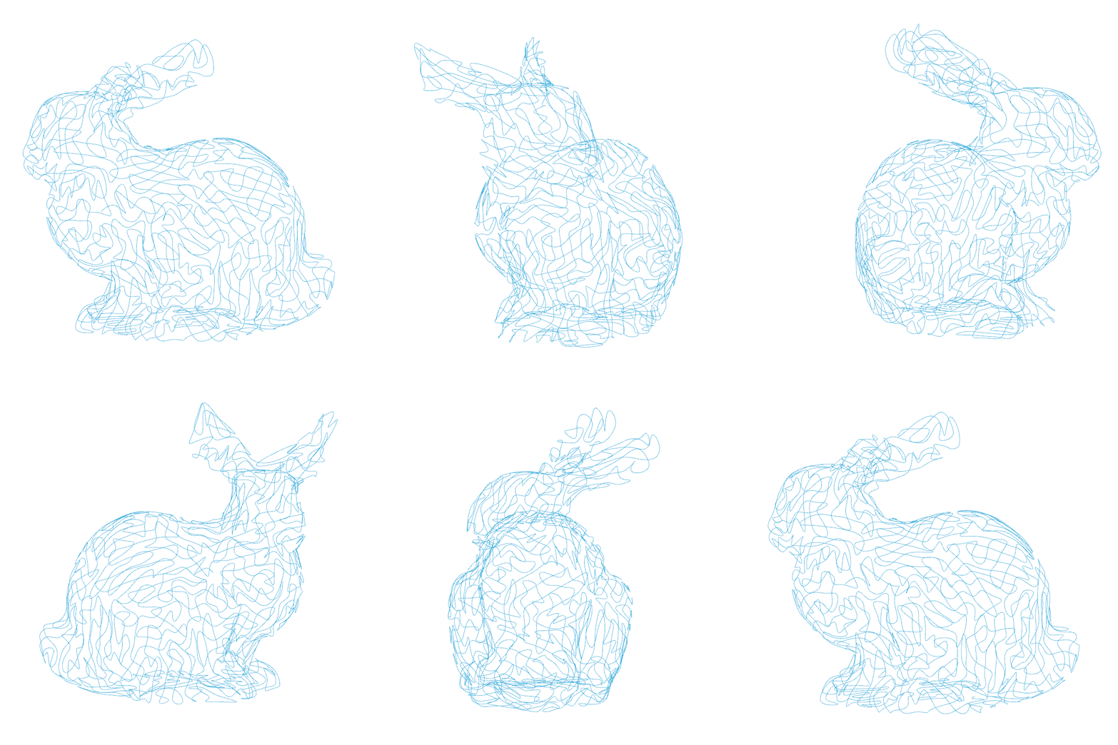
Additionally, Anemone can be used in conjunction with Kangaroo 2 to continuously subdivide the curve as it grows. The result is much smoother, as well as far more organic.

Of course the process can also be reversed, allowing the curve to flow seamlessly from one space to another.

Here are far more complex examples of growth simulations exploring various rules and parameters:
6.0 Developing Fractal Curves
In the interest of creating something a little more tangible, it is possible to increase the dimension of these curves. Recording the progressive iterations of a space filling curve allow us to generate what is essentially a space-filling surface. This new surface has the unique quality of being able to fill a three-dimensional space of any shape and size, while being a single surface. It of course also shares the same qualities as its source curves, where it keep increasing in surface area (and can do so indefinitely).

If you were to keep gradually (but indefinitely) increasing the area of a surface this way in a finite space, the result will be a two-dimensional surface seamlessly transforming into a three-dimensional volume.
6.1 Dragon’s Feet
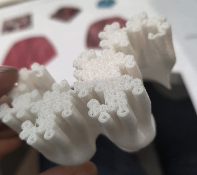
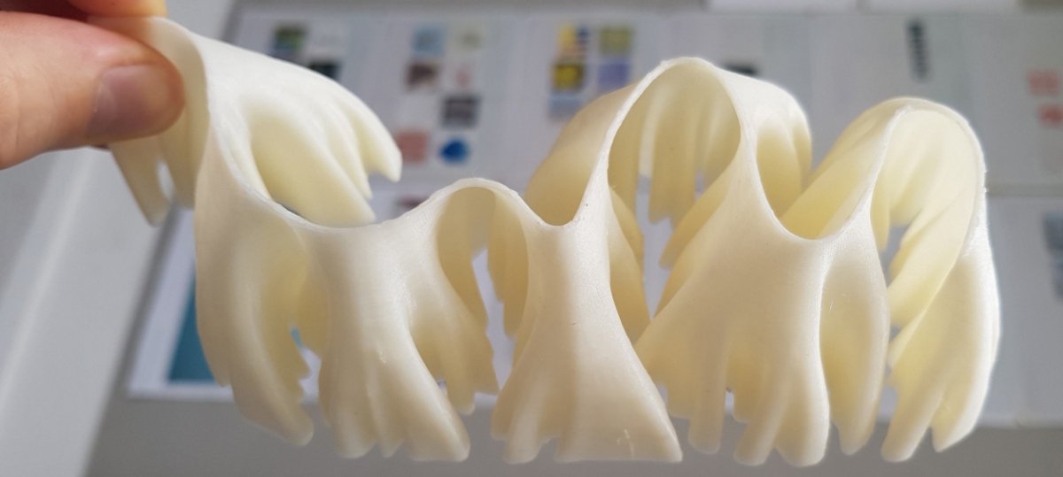
Here is an example of turning the dragon curve into a space-filling surface. Each iteration is recorded and offset in depth, all of which inform the generation of a surface that loosely flows through each of them. This was again achieved with Rhino and Grasshopper.
I don’t believe this geometry has a name beyond ‘the developing dragon curve’, so I’ve called it ‘Dragon’s Feet.’
Adding a little thickness to the model allow us to 3D print it.
6.2 Hilbert’s Curtain
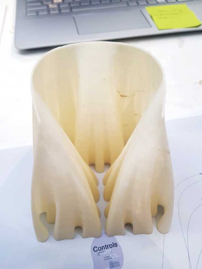
Here is the Hilbert Curve going through the same process, which I am aptly naming ‘Hilbert’s Curtain.’
3D Printing Space-Filling Curves with Henry Segerman at Numberphile:
‘Developing Fractal Curves’ by Geoffrey Irving & Henry Segerman:
6.3 Developing Whale Curve
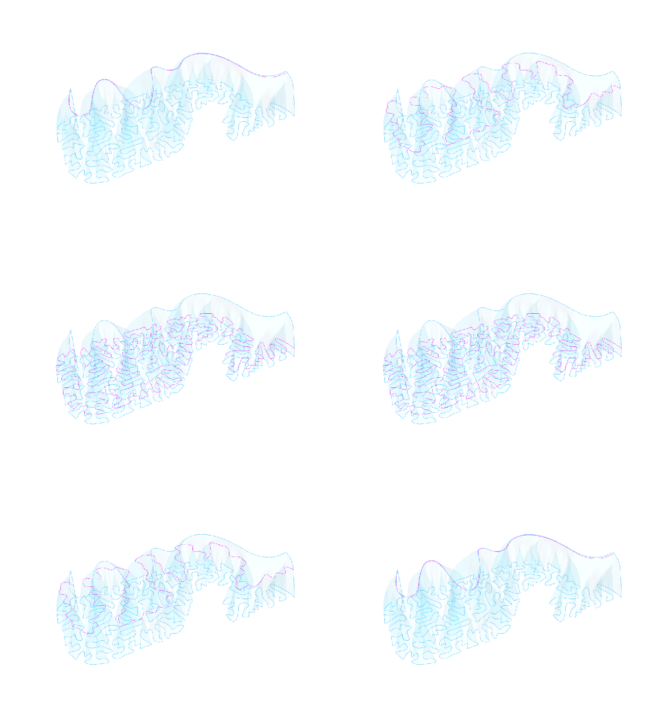
Unsurprisingly this can also be done with differentially grown curve. The respective difference being that this method fills a specific space in a less controlled manner.
In this case with Kangaroo 2 is used to grow a curve into the shape of a whale. Like before, each iteration is used to inform a single-surface geometry.


You really should give credit to Henry Segerman. He did this first.
Hi Nick could you share the grasshopper script of the planar differential growth?