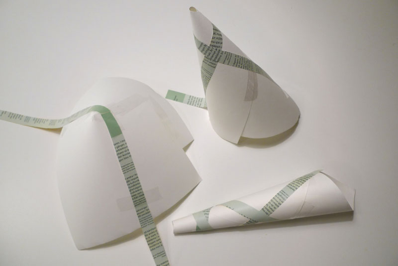
The main aspects of the Corn-Crete House system are the use of space, material efficiency and relationship to site. The way space is shaped influences human behaviour. According to a research paper done by KAYVAN MADANI NEJAD in 2007 the curvilinearity of interior design directly affects the way people feel inside them. It concluded that the more curvilinear a space is the more comfortable, safe, relaxed and friendly it feels. My project builds upon this argument. Research also shows that the concrete industry is a major environment pollutant. Cement is the most damaging ingredient. I am proposing a new system which will be using less concrete & less cement thanks to: 1) corn residues partially replacing aggregate making the structure lighter and more porous 2) casting around inflatables resulting in curvilinear architecture suitable for compression which requires less tensile strength.
Regarding my previous entries, it can be difficult to see how any of this has to do with architecture. In fact I know a few people who think studying fractals is pointless.
Admittedly I often struggle to explain to people what fractals are, let alone how they can influence the way buildings look. However, I believe that this post really sheds light on how these kinds of studies may directlyinfluence and enhance our understanding (and perhaps even the future) of our built environment.
On a separate note, I heard that a member of the architectural academia said “forget biomimicry, it doesn’t work.”
Firstly, I’m pretty sure Frei Otto would be rolling over in his grave.
Secondly, if someone thinks that biomimicry is useless, it’s because they don’t really understand what biomimicry is. And I think the same can be said regarding the study of fractals. They are closely related fields of study, and I wholeheartedly believe they are fertile grounds for architectural marvels to come.
7.0 Introduction to Shells
As far as classification goes, shells generally fall under the category of two-dimensional shapes. They are defined by a curved surface, where the material is thin in the direction perpendicular to the surface. However, assigning a dimension to certain shells can be tricky, since it kinda depends on how zoomed in you are.
A strainer is a good example of this – a two-dimensional gridshell. But if you zoom in, it is comprised of a series of woven, one-dimensional wires. And if you zoom in even further, you see that each wire is of course comprised of a certain volume of metal.
This is a property shared with many fractals, where their dimension can appear different depending on the level of magnification. And while there’s an infinite variety of possible shells, they are (for the most part) categorizable.
7.1 – Single Curved Surfaces
Analytic geometry is created in relation to Cartesian planes, using mathematical equations and a coordinate systems. Synthetic geometry is essentially free-form geometry (that isn’t defined by coordinates or equations), with the use of a variety of curves called splines. The following shapes were created via Synthetic geometry, where we’re calling our splines ‘u’ and ‘v.’
Uniclastic: Barrel Vault (Cylindrical paraboloid)
These curves highlight each dimension of the two-dimensional surface. In this case only one of the two ‘curves’ is actually curved, making this shape developable. This means that if, for example, it was made of paper, you could flatten it completely.
Uniclastic: Conoid (Conical paraboloid)
In this case, one of them grows in length, but the other still remains straight. Since one of the dimensions remains straight, it’s still a single curved surface – capable of being flattened without changing the area. Singly curved surfaced may also be referred to as uniclastic or monoclastic.
7.2 – Double Curved Surfaces
These can be classified as synclastic or anticlastic, and are non-developable surfaces. If made of paper, you could not flatten them without tearing, folding or crumpling them.
Synclastic: Dome (Elliptic paraboloid)
In this case, both curves happen to be identical, but what’s important is that both dimensions are curving in the same direction. In this orientation, the dome is also under compression everywhere.
The surface of the earth is double curved, synclastic – non-developable. “The surface of a sphere cannot be represented on a plane without distortion,” a topic explored by Michael Stevens: https://www.youtube.com/watch?v=2lR7s1Y6Zig
Anticlastic: Saddle (Hyperbolic paraboloid)
This one was formed by non-uniformly sweeping a convex parabola along a concave parabola. It’s internal structure will behave differently, depending on the curvature of the shell relative to the shape. Roof shells have compressive stresses along the convex curvature, and tensile stress along the concave curvature.
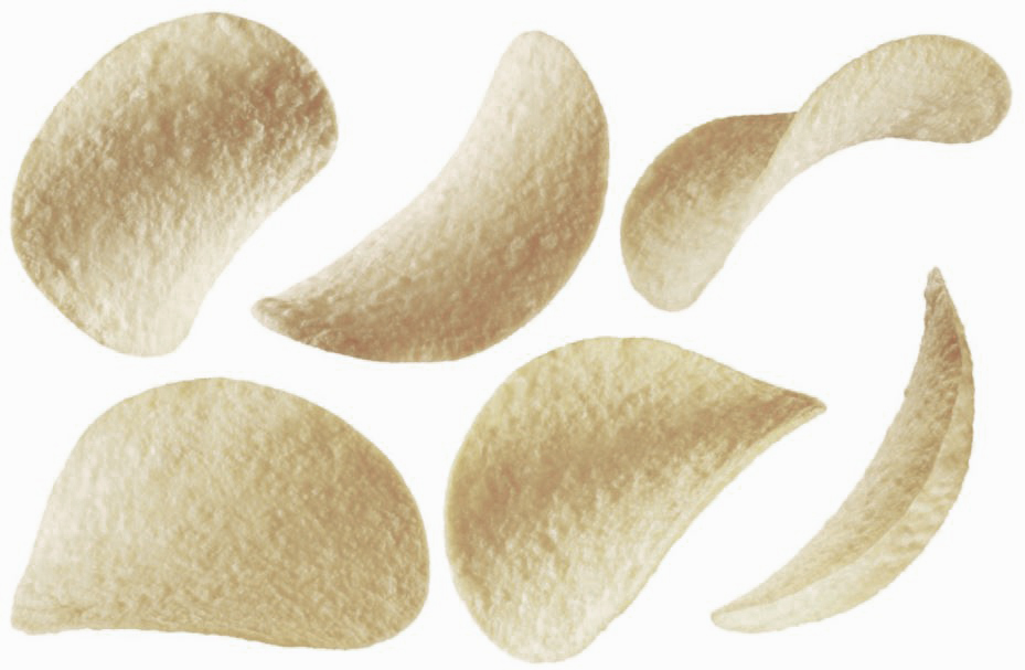
Kellogg’s potato and wheat-based stackable snack
Here is an example of a beautiful marriage of tensile and compressive potato and wheat-based anticlastic forces. Although I hear that Pringle cans are diabolically heinous to recycle, so they are the enemy.
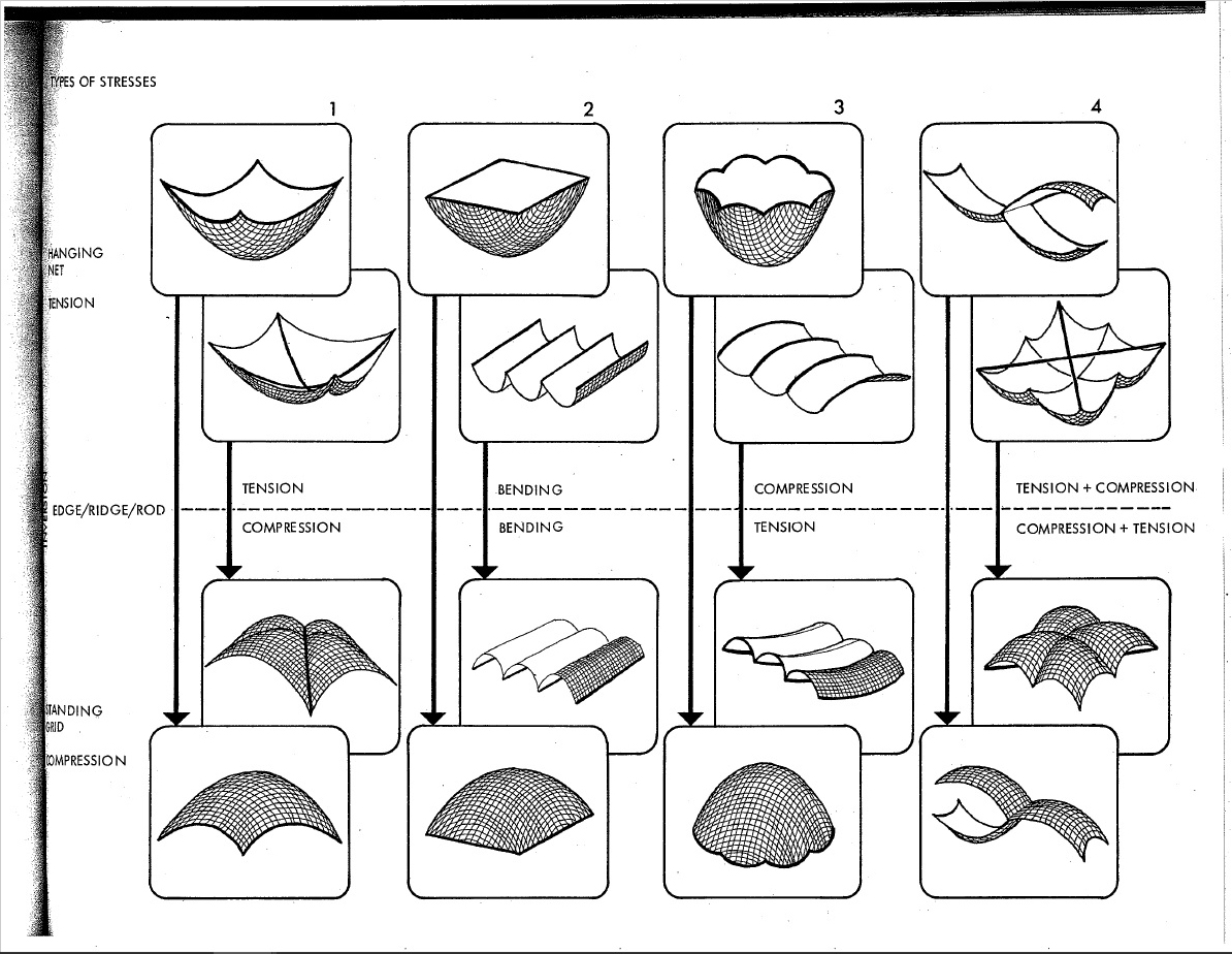
Structural Behaviour of Basic Shells [Source: IL 10 – Institute for Lightweight Structures and Conceptual Design]
7.3 – Translation vs Revolution
In terms of synthetic geometry, there’s more than one approach to generating anticlastic curvature:
Hyperbolic Paraboloid: Straight line sweep variation
This shape was achieved by sweeping a straight line over a straight path at one end, and another straight path at the other. This will work as long as both rails are not parallel. Although I find this shape perplexing; it’s double curvature that you can create with straight lines, yet non-developable, and I can’t explain it..
Ruled Surface & Surface of Revolution (Circular Hyperboloid)
The ruled surface was created by sliding a plane curve (a straight line) along another plane curve (a circle), while keeping the angle between them constant. The surfaces of revolution was simply made by revolving a plane curve around an axis. (Surface of translation also exist, and are similar to ruled surfaces, only the orientation of the curves is kept constant instead of the angle.)
Hyperboloid Generation [Source:Wikipedia]
The hyperboloid has been a popular design choice for (especially nuclear cooling) towers. It has excellent tensile and compressive properties, and can be built with straight members. This makes it relatively cheap and easy to fabricate relative to it’s size and performance.
These are singly curved curves, although that does sound confusing. A simple way to understand what geodesic curves are, is to give them a width. As previously explored, we know that curves can inhabit, and fill, two-dimensional space. However, you can’t really observe the twists and turns of a shape that has no thickness.
Conic Plank Lines (Source: The Geometry of Bending)
A ribbon is essentially a straight line with thickness, and when used to follow the curvature of a surface (as seen above), the result is a plank line. The term ‘plank line’ can be defined as a line with an given width (like a plank of wood) that passes over a surface and does not curve in the tangential plane, and whose width is always tangential to the surface.
Since one-dimensional curves do have an orientation in digital modeling, geodesic curves can be described as the one-dimensional counterpart to plank lines, and can benefit from the same definition.
For simplicity, here’s a basic grid set up on a flat plane:
Basic geodesic curves on a plane
We start by defining two points anywhere along the edge of the surface. Then we find the geodesic curve that joins the pair. Of course it’s trivial in this case, since we’re dealing with a flat surface, but bear with me.
Initial set of curves
We can keep adding pairs of points along the edge. In this case they’re kept evenly spaced and uncrossing for the sake of a cleaner grid.
Addition of secondary set of curves
After that, it’s simply a matter of playing with density, as well as adding an additional set of antagonistic curves. For practicality, each set share the same set of base points.
Grid with independent sets
He’s an example of a grid where each set has their own set of anchors. While this does show the flexibility of a grid, I think it’s far more advantageous for them to share the same base points.
8.2 – Basic Gridshells
The same principle is then applied to a series of surfaces with varied types of curvature.
Uniclastic: Barrel Vault Geodesic Gridshell
First comes the shell (a barrel vault in this case), then comes the grid. The symmetrical nature of this surface translates to a pretty regular (and also symmetrical) gridshell. The use of geodesic curves means that these gridshells can be fabricated using completely straight material, that only necessitate single curvature.
Uniclastic: Conoid Geodesic Gridshell
The same grid used on a conical surface starts to reveal gradual shifts in the geometry’s spacing. The curves always search for the path of least resistance in terms of bending.
Synclastic: Dome Geodesic Gridshell
This case illustrates the nature of geodesic curves quite well. The dome was free-formed with a relatively high degree of curvature. A small change in the location of each anchor point translates to a large change in curvature between them. Each curve looks for the shortest path between each pair (without leaving the surface), but only has access to single curvature.
Anticlastic: Saddle Geodesic Gridshell
Structurally speaking, things get much more interesting with anticlastic curvature. As previously stated, each member will behave differently based on their relative curvature and orientation in relation to the surface. Depending on their location on a gridshell, plank lines can act partly in compression and partly in tension.
On another note:
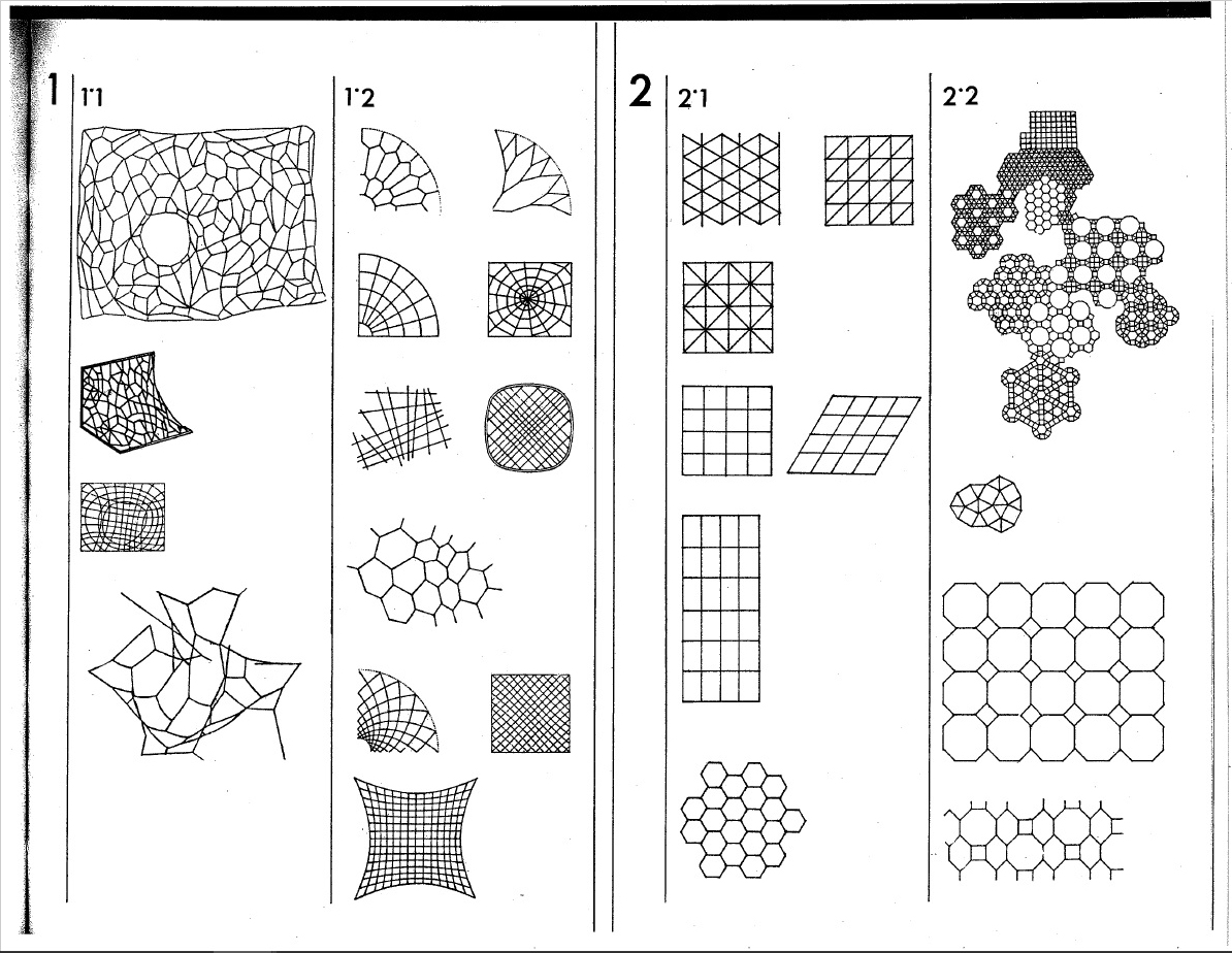
While geodesic curves make it far more practical to fabricate shells, they are not a strict requirement. Using non-geodesic curves just means more time, money, and effort must go into the fabrication of each component. Furthermore, there’s no reason why you can’t use alternate grid patterns. In fact, you could use any pattern under the sun – any motif your heart desires (even tessellated puppies.)
Alternate Gridshell Patterns [Source: IL 10 – Institute for Lightweight Structures and Conceptual Design]
Here are just a few of the endless possible pattern. They all have their advantages and disadvantages in terms of fabrication, as well as structural potential.
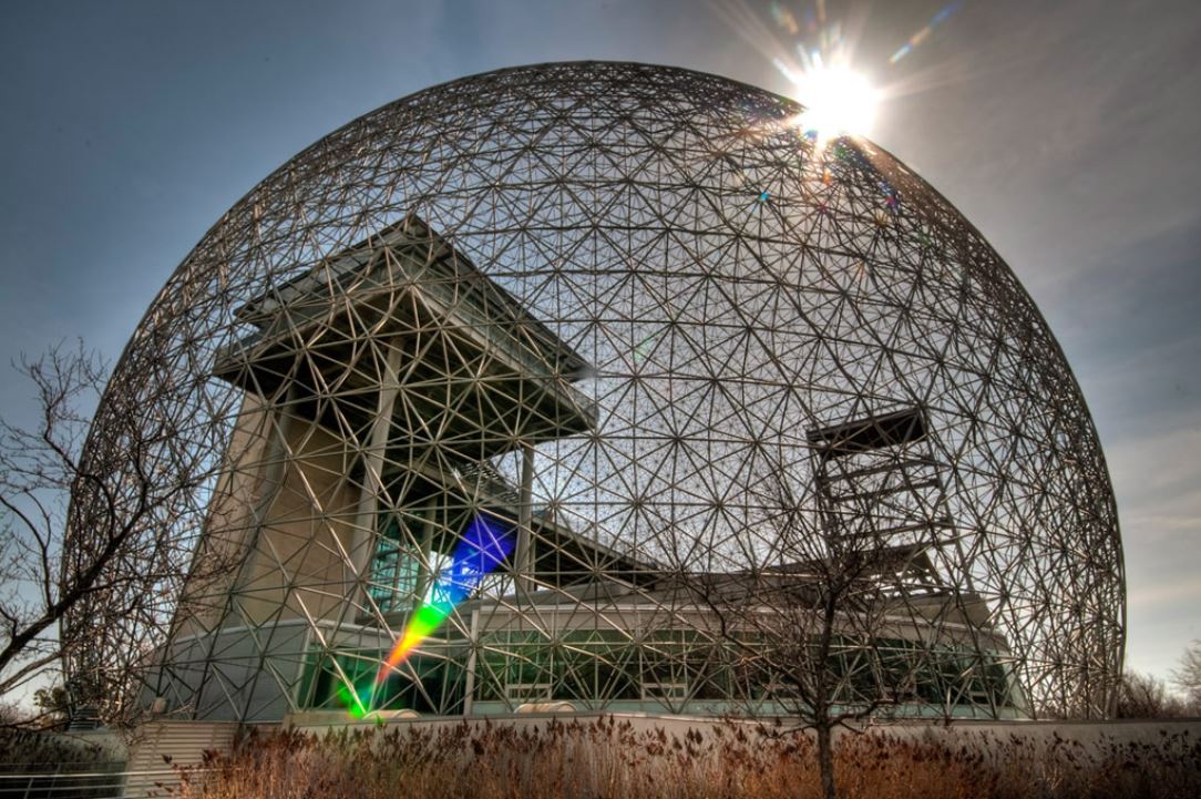
Biosphere Environment Museum – Canada
Gridshells with large amounts of triangulation, such as Buckminster Fuller’s geodesic spheres, typically perform incredibly well structurally. These structure are also highly efficient to manufacture, as their geometry is extremely repetitive.
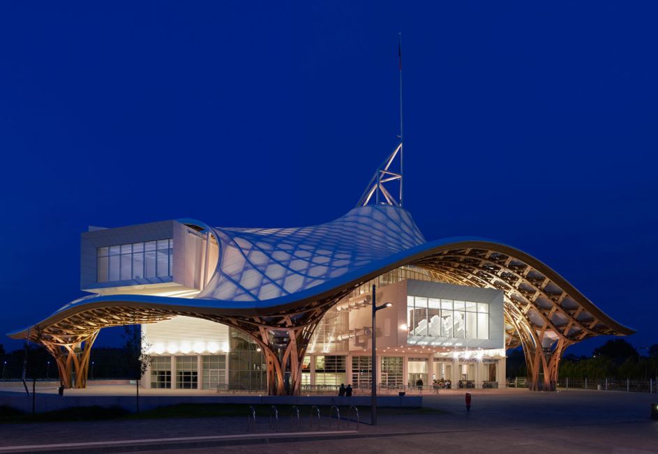
Centre Pompidou-Metz – France
Gridshells with highly irregular geometry are far more challenging to fabricate. In this case, each and every piece had to be custom made to shape; I imagine it must have costed a lot of money, and been a logistical nightmare. Although it is an exceptionally stunning piece of architecture (and a magnificent feat of engineering.)
8.3 – Gridshell Construction
In our case, building these shells is simply a matter of converting the geodesic curves into planks lines.
Hyperbolic Paraboloid: Straight Line Sweep Variation With Rotating Plank Line Grid
The whole point of using them in the first place is so that we can make them out of straight material that don’t necessitate double curvature. This example is rotating so the shape is easier to understand. It’s grid is also rotating to demonstrate the ease at which you can play with the geometry.
Hyperbolic Paraboloid: Flattened Plank Lines With Junctions
This is what you get by taking those plank lines and laying them flat. In this case both sets are the same because the shell happens to the identicall when flipped. Being able to use straight material means far less labour and waste, which translates to faster, and or cheaper, fabrication.
An especially crucial aspect of gridshells is the bracing. Without support in the form of tension ties, cable ties, ring beams, anchors etc., many of these shells can lay flat. This in and of itself is pretty interesting and does lends itself to unique construction challenges and opportunities. This isn’t always the case though, since sometimes it’s the geometry of the joints holding the shape together (like the geodesic spheres.) Sometimes the member are pre-bent (like Pompidou-Metz.) Although pre-bending the timber kinda strikes me as cheating thought.. As if it’s not a genuine, bona fide gridshell.
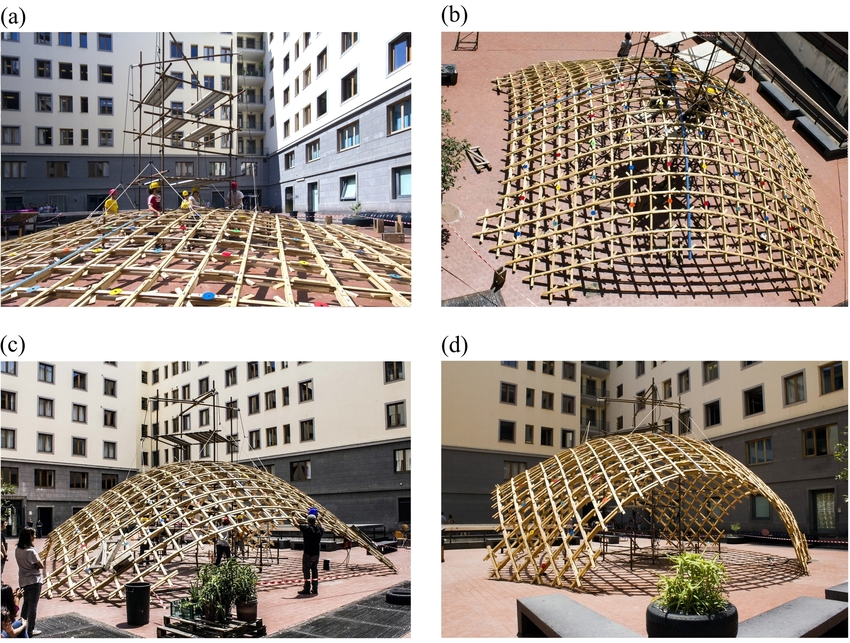
Toledo Gridshell 2.0. Construction Process [source: Timber gridshells – Numerical simulation, design and construction of a full scale structure]
This is one of the original build method, where the gridshell is assembled flat, lifted into shape, then locked into place.
9.0 Form Finding
Having studied the basics makes exploring increasingly elaborate geometry more intuitive. In principal, most of the shells we’ve looked are known to perform well structurally, but there are strategies we can use to focus specifically on performance optimization.
9.0 – Minimal Surfaces
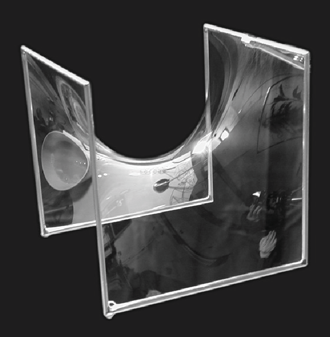
These are surfaces that are locally area-minimizing – surfaces that have the smallest possible area for a defined boundary. They necessarily have zero mean curvature, i.e. the sum of the principal curvatures at each point is zero. Soap bubbles are a great example of this phenomenon.
Hyperbolic Paraboloid Soap Bubble [Source: Serfio Musmeci’s “Froms With No Name” and “Anti-Polyhedrons”]Soap film inherently forms shapes with the least amount of area needed to occupy space – that minimize the amount of material needed to create an enclosure. Surface tension has physical properties that naturally relax the surface’s curvature.
Kangaroo2 Physics: Surface Tension Simulation
We can simulate surface tension by using a network of curves derived from a given shape. Applying varies material properties to the mesh results in a shape that can behaves like stretchy fabric or soap. Reducing the rest length of each of these curves (while keeping the edges anchored) makes them pull on all of their neighbours, resulting in a locally minimal surface.
Here are a few more examples of minimal surfaces you can generate using different frames (although I’d like stress that the possibilities are extremely infinite.) The first and last iterations may or may not count, depending on which of the many definitions of minimal surfaces you use, since they deal with pressure. You can read about it in much greater detail here: https://tinyurl.com/ya4jfqb2
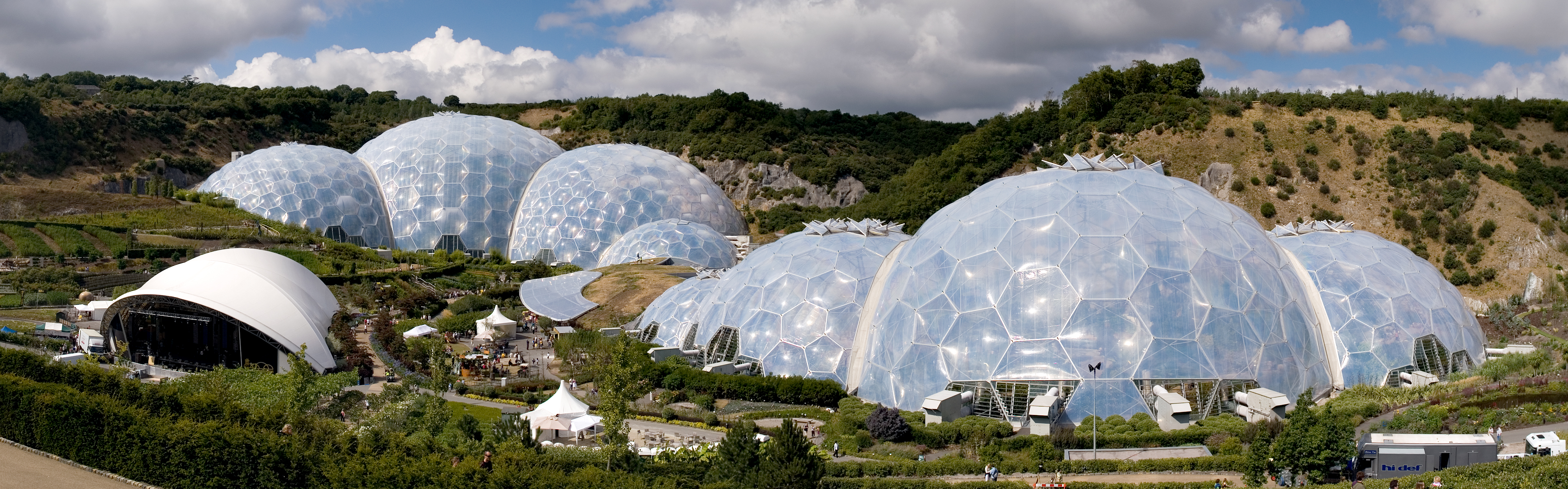
The Eden Project – United Kingdom
Here we have one of the most popular examples of minimal surface geometry in architecture. The shapes of these domes were derived from a series of studies using clustered soap bubbles. The result is a series of enormous shells built with an impressively small amount of material.
Triply periodic minimal surfaces are also a pretty cool thing (surfaces that have a crystalline structure – that tessellate in three dimensions):
Another powerful method of form finding has been to let gravity dictate the shapes of structures. In physics and geometry, catenary (derived from the Latin word for chain) curves are found by letting a chain, rope or cable, that has been anchored at both end, hang under its own weight. They look similar to parabolic curves, but perform differently.
Kangaroo2 Physics: Catenary Model Simulation
A net shown here in magenta has been anchored by the corners, then draped under simulated gravity. This creates a network of hanging curves that, when converted into a surface, and mirrored, ultimately forms a catenary shell. This geometry can be used to generate a gridshell that performs exceptionally well under compression, as long as the edges are reinforced and the corners are braced.
While I would be remiss to not mention Antoni Gaudí on the subject of catenary structure, his work doesn’t particularly fall under the category of gridshells. Instead I will proceed to gawk over some of the stunning work by Frei Otto.
Of course his work explored a great deal more than just catenary structures, but he is revered for his beautiful work on gridshells. He, along with the Institute for Lightweight Structures, have truly been pioneers on the front of theoretical structural engineering.
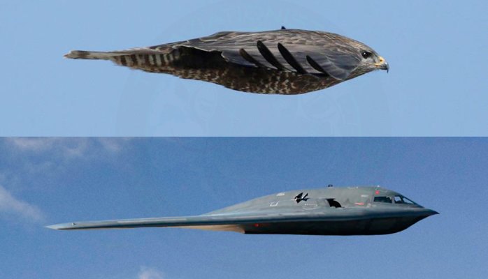
9.3 – Biomimicry in Architecture
There are a few different terms that refer to this practice, including biomimetics, bionomics or bionics. In principle they are all more or less the same thing; the practical application of discoveries derived from the study of the natural world (i.e. anything that was not caused or made by humans.) In a way, this is the fundamental essence of the scientific method: to learn by observation.
Example of Biomimicry
Frei Otto is a fine example of ecological literacy at its finest. A profound curiosity of the natural world greatly informed his understanding of structural technology. This was all nourished by countless inquisitive and playful investigations into the realm of physics and biology. He even wrote a series of books on the way that the morphology of bird skulls and spiderwebs could be applied to architecture called Biology and Building. His ‘IL‘ series also highlights a deep admiration of the natural world.
Of course he’s the not the only architect renown their fascination of the universe and its secrets; Buckminster Fuller and Antoni Gaudí were also strong proponents of biomimicry, although they probably didn’t use the term (nor is the term important.)
Gaudí’s studies of nature translated into his use of ruled geometrical forms such as hyperbolic paraboloids, hyperboloids, helicoids etc. He suggested that there is no better structure than the trunk of a tree, or a human skeleton. Forms in biology tend to be both exceedingly practical and exceptionally beautiful, and Gaudí spent much of his life discovering how to adapt the language of nature to the structural forms of architecture.
Fractals were also an undisputed recurring theme in his work. This is especially apparent in his most renown piece of work, the Sagrada Familia. The varying complexity of geometry, as well as the particular richness of detail, at different scales is a property uniquely shared with fractal nature.
Antoni Gaudí and his legacy are unquestionably one of a kind, but I don’t think this is a coincidence. I believe the reality is that it is exceptionally difficult to peruse biomimicry, and especially fractal geometry, in a meaningful way in relation to architecture. For this reason there is an abundance of superficial appropriation of organic, and mathematical, structures without a fundamental understanding of their function. At its very worst, an architect’s approach comes down to: ‘I’ll say I got the structure from an animal. Everyone will buy one because of the romance of it.”
That being said, modern day engineers and architects continue to push this envelope, granted with varying levels of success. Although I believe that there is a certain level of inevitability when it comes to how architecture is influenced by natural forms. It has been said that, the more efficient structures and systems become, the more they resemble ones found in nature.
Euclid, the father of geometry, believed that nature itself was the physical manifestation of mathematical law. While this may seems like quite a striking statement, what is significant about it is the relationship between mathematics and the natural world. I like to think that this statement speaks less about the nature of the world and more about the nature of mathematics – that math is our way of expressing how the universe operates, or at least our attempt to do so. After all, Carl Sagan famously suggested that, in the event of extra terrestrial contact, we might use various universal principles and facts of mathematics and science to communicate.
The study of fractals is an intensely vast topic. So much so that I’m convinced you could easily spend several lifetimes studying them. That being said, I chose to focus specifically on single-curve geometry. But, keep in mind that I’m only really scratching the surface of what there is to explore.
4.0 Classic Space-Filling
Inspired by Georg Cantor’s research on infinity near the end of the 19th century, mathematicians were interested in finding a mapping of a one-dimensional line into two-dimensional space – a curve that will pass through through every single point in a given space.
Jeffrey Ventrella writes that “a space-filling curve can be described as a continuous mapping from a lower-dimensional space into a higher-dimensional space.” In other words, an initial one-dimensional curve is developed to increase its length and curvature – the amount of space in occupies in two dimensions. And in the mathematical world, where a curve technically has no thickness and space is infinitely vast, this can be done indefinitely.
4.1 Early Examples
In 1890, Giuseppe Peano discovered the first of what would be called space-filing curves:
4 Iterations of the Peano Curve
An initial ‘curve’ is drawn, then each element of the curve is replace by the whole thing. Here it is done four times, and it’s easy to imagine how you can keep doing this over and over again. One would think that if you kept doing this indefinitely, this one-dimensional curve would eventually fill all of two-dimensional space and become a surface. However it can’t, since it technically has no thickness. So it will be as close as you can get to a surface, without actually being a surface (I think.. I’m not that sure..)
A year later, David Hilbert followed with his slightly simpler space-filing curve:
8 Iterations of the Hilbert Curve
In 1904, Helge von Koch describes a single complex continuous curve, generated with rudimentary geometry.
7 Iterations of the Koch Curve
Around 1967, NASA physicists John Heighway, Bruce Banks, and William Harter discovered what is now commonly known as the Dragon Curve.
13 Iterations of the Dragon Curve
4.2 Later Examples
You may have noticed that some of these curves are better at filling space than others, and this is related to their dimensional measure. They fall under the category of fractals because they’re neither one-dimensional, nor two-dimensional, but sit somewhere in between. For these examples, their dimension is often defined by exactly how much space they fill when iterated infinitely.
While these are some of the earliest space-filling curves to be discovered, they are just a handful of the likely endless different variations that are possible. Jeffrey Ventrella spent over twenty-five years exploring fractal curves, and has illustrated over 200 hundred of them in his book ‘Brain-Filling Curves, A Fractal Bestiary.’ They are organised according to a taxonomy of fractal curve families, and are shown with a unique genetic code.
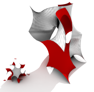
Incidentally, in an attempt to recreate one of the fractals I found in Jeffery Ventrella’s book, I accidentally created a slightly different fractal. As far as I’m concerned, I’ve created a new fractal and am unofficially naming it ‘Nicolino’s Quatrefoil.’ The following was created in Rhino and Grasshopper, in conjunction Anemone.
5 Iterations of Nicolino’s Quatrefoil
You can find beautifully animated space-filling curves here:
As an object, it seems perplexingly difficult to categorize. It is a single, one-dimensional, curve that is ‘bent’ in space following simple, repeating rules. Following the same logic as the original Hilbert Curve, we know that this can be done indefinitely, but this time it is transforming into a volume instead of a surface. (Ignoring the fact that it is represented with a thickness) It is a one-dimensional curve transforming into a three-dimensional volume, but is never a two-dimensional surface? As you keep iterating it, its dimension gradually increases from 1 to eventually 3, but will never, ever, ever be 2??
Nevertheless this does actually support a statement I made in my last post suggesting “…there is no ‘first’ or ‘second’ dimension. It’s a bit like pouring three cups of water into a vase and asking someone which cup is the first one. The question doesn’t even make sense…“
5.0 Avant-Garde Space-Filling
In the case of the original space-filling curve, the goal was to fill all of infinite space. However the fundamental behaviour of these curves change quite drastically when we start to play with the rules used to generate them. For starters, they do not have to be so mathematically tidy, or geometrically pure. The following curves can be subdivided infinitely, making them true space-filling curves. But, what makes them special is the ability to control the space-filling process, whereas the original space-filling curves offer little to no artistic license.
5.1 The Traveling Salesman Problem
Let’s say that we change the criteria, from passing through every single point in space, to passing only through the ones we choose. This now becomes a well documented computational problem that has immediate ‘real world’ applications.
Our figurative traveling salesman wishes to travel the country selling his goods in as many cities as he can. In order to maximize his net profit, he must make his journey as short as possible, while of course still visiting every city on his list. His best possible route becomes exponentially more challenging to work out, as even just a handful of cities can generate thousands of permutations.
There are a variety of different strategies to tackle this problem, a few of which are described here:
The result is ultimately a single curve, filling a space in a uniquely controlled fashion. This method can be used to create single-lined drawings based on points extracted from Voronoi diagrams, a topic explored by Arjan Westerdiep:
This illustration, commissioned by Bill Cook at University of Waterloo, is a solution to the Traveling Salesman Problem.
5.2 Differential Growth
If we let physics (rather than math) dictate the growth of the curve, the result becomes more organic and less controlled.
In this example Rhino is used with Grasshopper and Kangaroo 2. A curve is drawn on a plain, broken into segments, then gradually increased in length. As long as the curve is not allowed to cross itself (which is achieved here with ‘Collision Spheres’), the result is a curve that is pretty good at uniformly filling space.
The geometry doesn’t even have to be bound by a planar surface; It can be done on any two-dimensional surface (or in three-dimensions (even higher spacial dimensions I guess..)).
Additionally, Anemone can be used in conjunction with Kangaroo 2 to continuously subdivide the curve as it grows. The result is much smoother, as well as far more organic.
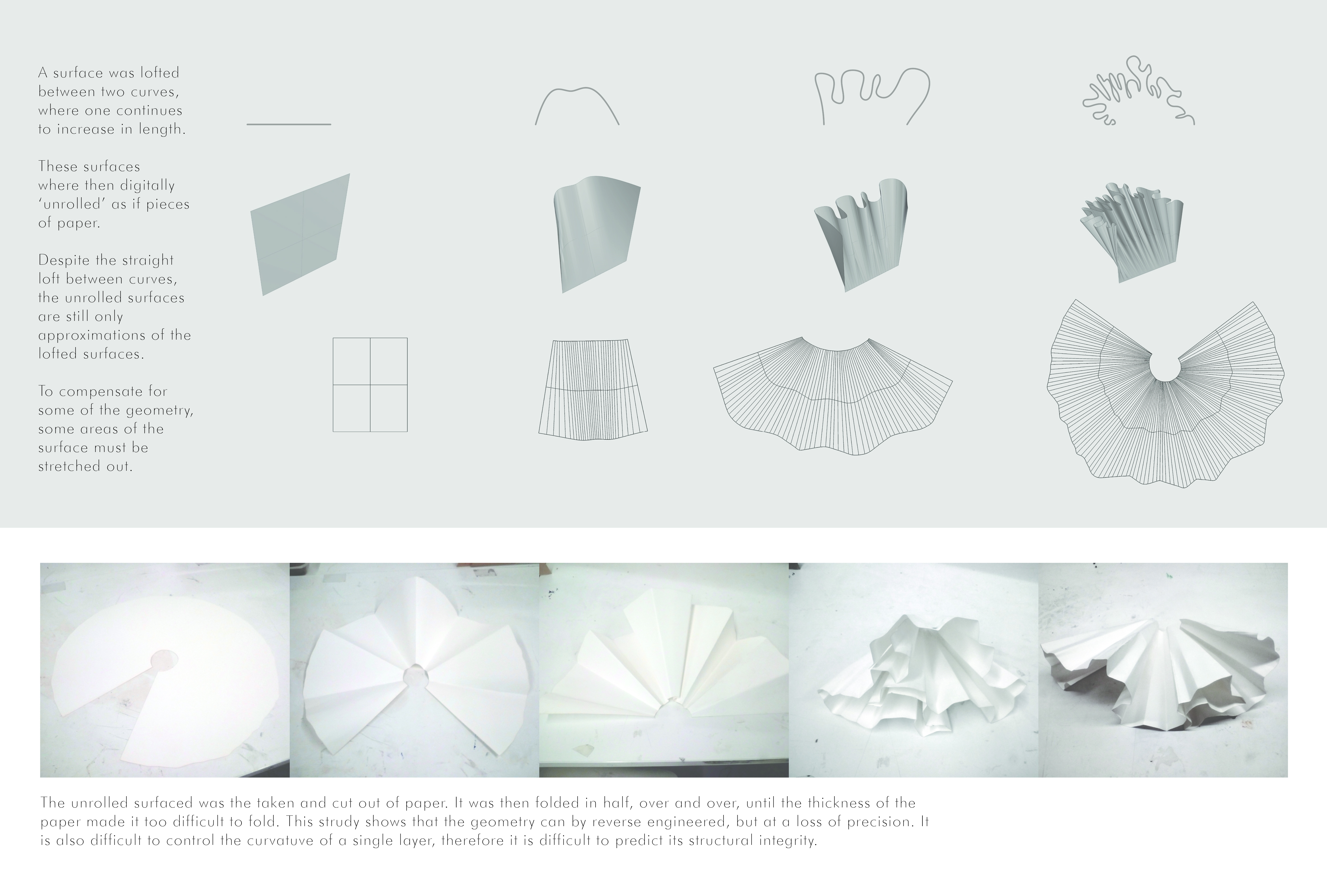
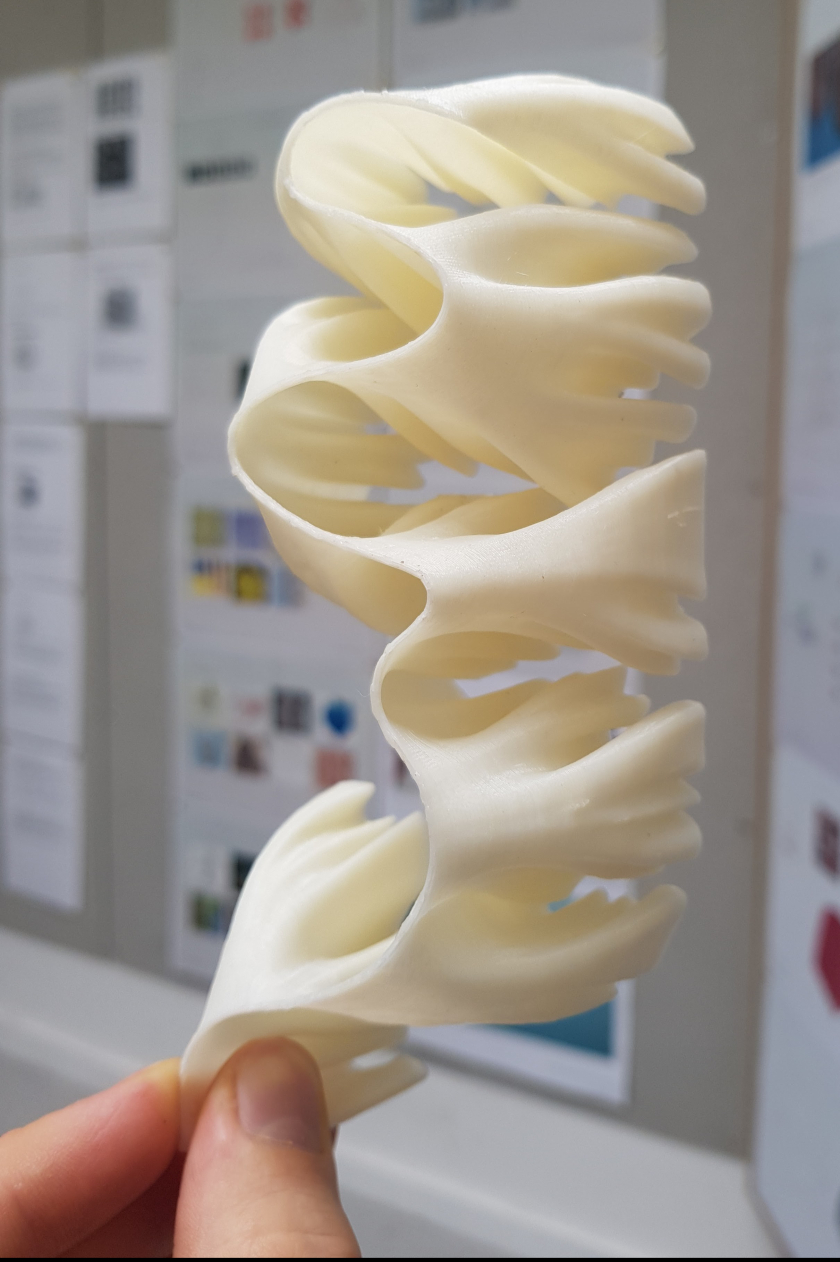
In the interest of creating something a little more tangible, it is possible to increase the dimension of these curves. Recording the progressive iterations of a space filling curve allow us to generate what is essentially a space-filling surface. This new surface has the unique quality of being able to fill a three-dimensional space of any shape and size, while being a single surface. It of course also shares the same qualities as its source curves, where it keep increasing in surface area (and can do so indefinitely).
Surface Unrolling Study
If you were to keep gradually (but indefinitely) increasing the area of a surface this way in a finite space, the result will be a two-dimensional surface seamlessly transforming into a three-dimensional volume.
6.1 Dragon’s Feet
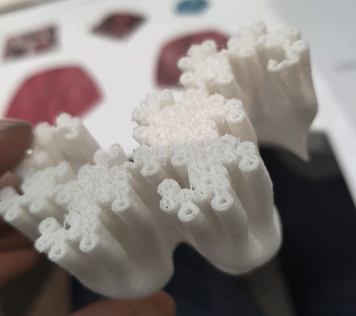
Here is an example of turning the dragon curve into a space-filling surface. Each iteration is recorded and offset in depth, all of which inform the generation of a surface that loosely flows through each of them. This was again achieved with Rhino and Grasshopper.
I don’t believe this geometry has a name beyond ‘the developing dragon curve’, so I’ve called it ‘Dragon’s Feet.’
Adding a little thickness to the model allow us to 3D print it.
Unsurprisingly this can also be done with differentially grown curve. The respective difference being that this method fills a specific space in a less controlled manner.
In this case with Kangaroo 2 is used to grow a curve into the shape of a whale. Like before, each iteration is used to inform a single-surface geometry.
Iterative Steps of the Differentially Grown Whale Curve
Frequently occuring in nature, minimal surfaces are defined as surfaces with zero mean curvature. These surfaces originally arose as surfaces that minimized total surface area subject to some constraint. Physical models of area-minimizing minimal surfaces can be made by dipping a wire frame into a soap solution, forming a soap film, which is a minimal surface whose boundary is the wire frame.
The thin membrane that spans the wire boundary is a minimal surface of all possible surfaces that span the boundary, it is the one with minimal energy. One way to think of this “minimal energy” is that to imagine the surface as an elastic rubber membrane: the minimal shape is the one that in which the rubber membrane is the most relaxed.
A minimal surface parametrized as x=(u,v,h(u,v)) therefore satisfies Lagrange`s equation
This year`s research focuses on triply periodic minimal surfaces (TPMS). A TPMS is a type of minimal surface which is invariant under a rank-3 lattice of translations. In other words, a TPMS is a surfaces which, through mirroring and rotating in 3D space, can form an infinite labyrinth. TPMS are of particular relevance in natural sciences, having been observed in observed as biological membranes, as block copolymers, equipotential surfaces in crystals, etc.
From a mathematical standpoint, a TPMS is the most interesting type of surface, as all connected RPMS have genus >=3, and in every lattice there exist orientable embedded TPMS of every genus >=3. Embedded TPMS are orientable and divide space into disjoint sub-volumes. If they are congruent the surface is said to be a balance surface.
The first examples of TPMS were the surfaces described by Schwarz in 1865, followed by a surface described by his student Neovius in 1883. In 1970 Alan Schoen, a then NASA scientist, described 12 more TPMS, and in 1989 H. Karcher proved their existence.
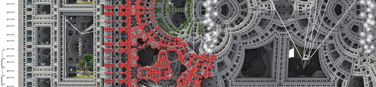
The first part of my research focuses on understanding TPMS geometry using a generation method that uses a marching cubes algorithm to find the results of the implicit equtions describing each particular type of TMPS. The resulting points form a mesh that describes the geometry.
Schwartz_P surface
Neovius surface
Gyroid surface
Generated from mathematical equations, these diagrams show the plotting of functions with different domains. Above, the diagrams on the left illustrate the process of forming a closed TMPS, starting from a domain of 0.5, which generates an elementary cell, which is mirrored and rotate 7 times to form a closed TPMS. A closed TMPS can also be approximated by changing the domain of the function to 1.
The diagrams below show some examples generating a TMPS from a function with a domain of 2. The views are front, top and axonometric.
This method of approximating a TPMS is high versatile, useful in understanding the geometry, offsetting the surfaces and changing the bounding box of the lattice in which the surface is generated. In other words, trimming the surface and isolating parts of the surface. However, the resulting topology is unsuitable for fabrication purposes, as the generated mesh is unclean, being composed of irregular polygons consisting of triangulations, quads and hexagons.
The following diagrams show the mesh topology for a Gyroid surface, offset studies and trimming studies.
For fabrication purposes, my proposed method for computationally simulating a TPMS is derived from discrete differential geometry, relying on the use of Kangaroo Physics, a Grasshopper plugin for modeling tensile membranes. Bearing in mind that a TPMS has 6 edge conditions, a planar hexagonal mesh is placed within the space defined by a certain TPMS`s edge conditions. The edge conditions are interpreted as Nurbs curves. Constructed from 6 predefined faces, the initial planar hexagonal mesh, together with the curves defining the surface boundaries are split into the same number of subdivisions. The subdivision algorithm used on the mesh is WeaveBird`s triangular subdivision. The points resulted from the curve division are ordered so that they match the subdivided mesh`s edges, or its naked vertices. The naked vertices are then moved in the corresponding points on the curve, resulting in a new mesh describing a triply periodic surface, but not a minimal one. From this point, Kangaroo Physics is used to find the minimal surface for the given mesh parameters, resulting in a TPMS.
Sequential diagram showing the generation of a Schwartz_P surfaces using the above method.
A Gyroid surface approximated with the above method
This approach towards approximating a TPMS leads to a study in the change of boundary conditions, gaining control over the geometry. The examples below present various gyroid distorsions generated by changing the boundary conditions.
Being able to control the boundary conditions defining a gyroid, or any TPMS, opens up to form optimization through genetic algorithms. Here, various curvatures for the edge conditions have been tested with regards to solar gain, using Galapagos for Grasshopper.
The following examples show some patterns generated by different topologies of the starting mesh.
All living organisms are composed of cells, and cells are fluid-filled spaces surrounded by an envelope of little material- cell membrane. Frei Otto described this kind of structure as pneus.
From first order, peripheral conditions or the packing configuration spatially give rise to specific shapes we see on the second and third order.
This applies to most biological instances. On a larger scale, the formation of beehives is a translated example of the different orders of ‘pneu’.
Interested to see the impact of lattice configuration on the forms, I moved on to digital physics simulation with Kangaroo 2 (based on a script by David Stasiuk). The key parameters involved for each lattice configuration are:
Inflation pressure in spheres
Collision force between the spheres
Collision force of spheres and bounding box
Surface tension of spheres
Weight.
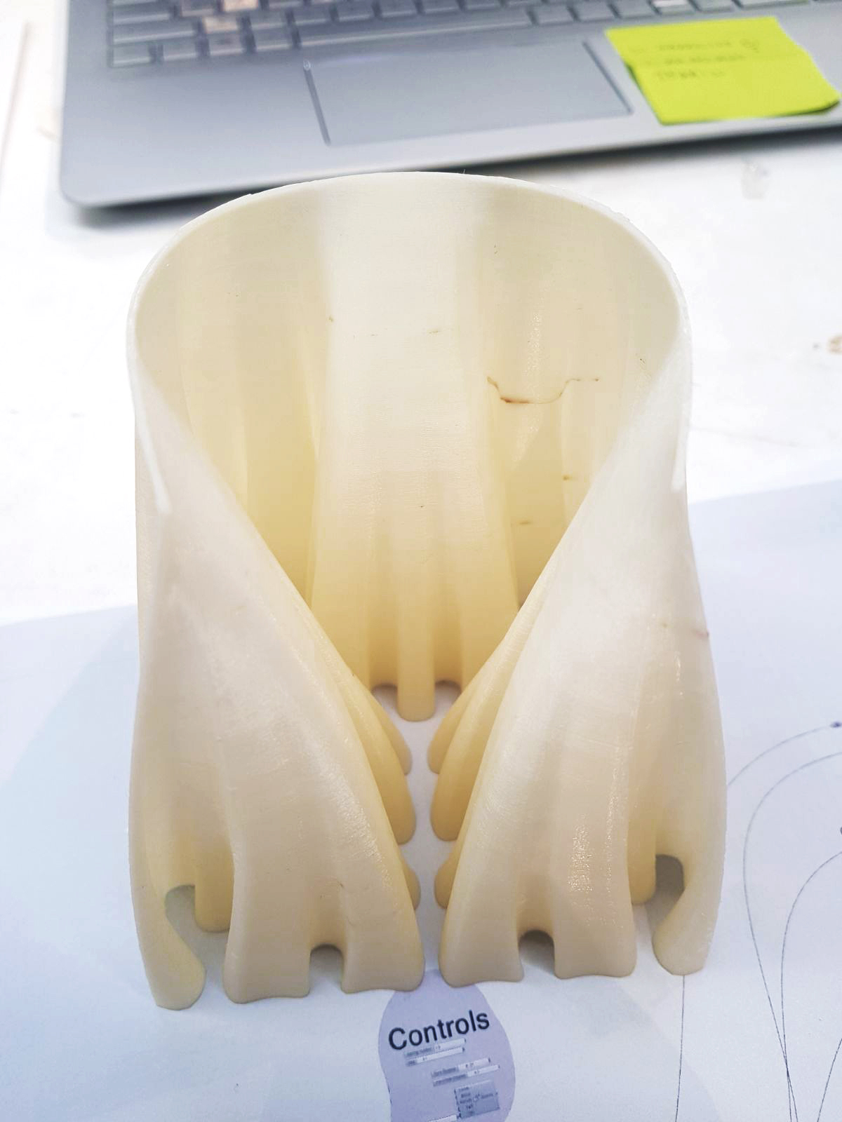
Physical exploration is also done to understand pneumatic behaviors and their parameters.
This followed by 3D pneumatic space packing. Spheres in different lattice configuration is inflated, and then taken apart to examine the deformation within. This process can be thought of as the growing process of seeds or pips in fruits such as pomegranates and citrus under hydrostatic pressure within its skin; and dissections of these fruits.
As the spheres take the peripheral conditions, the middles ones which are surrounded by spheres transformed into Rhombic dodecahedron, Trapezoid Rhombic dodecahedron and diamond respectively in Hex Grid, FCC Grid, and Square Grid. The spheres at the boundary take the shape of the bounding box hence they are more fully inflated(there are more spaces in between spheres and bounding box for expansion).
Physical experimentation has been done on inflatables structures. The following shows some of the outcome on my own and during an Air workshop in conjunction with Playweek led by Will Mclean and Laylac Shahed.
To summarize, pneumatic structures are forms wholly or mainly stabalised by either
– Pressurised difference in gas. Eg. Air structure or aerated foam structures
– liquid/hydrostatic pressure. Eg. Plant cells
– Forces between materials in bulk. Eg. Beehive, Fruits seeds/pips
There is a distinct quality of unpredictability and playfulness that pneumatic structures could offer. The jiggly nature of inflatables, the unpredictability resulted from deformation by compression and its lightweightness are intriguing. I will call them as pneumatic behaviour. I will continually explore what pneumatic materials and assembly of them could offer spatially in Brief 02. Digital simulations proved to be helpful in expressing the dynamic behaviours of pneumatic structures too, which I intend to continue.
I have been researching Miura pattern origami as a structural solution for rapidly deployable structures. Miura ori are interesting as structures due to their ability to develop from a flat surface to a 3D form, and become fully rigid, with no degrees of freedom, once constrained at certain points. Physical and digital experiments with Miura Ori have taught me that certain topographies can be generated by developing a modified Miura pattern. With the help of Tomohiro Tachi’s excellent research on the subject of curved Miura ori, including his Freeform Origami simulator (http://www.tsg.ne.jp/TT/index.html) I have learned that Miura ori surfaces that curve in the X and Y axes can be generated by modifying the tessellating components, however these modifications require some flexibility in the material, or looseness of the hinges. As a system for a rapidly deployable structure, I am most interested in the potential for the modified Miura ori to work as a structure built with cheap, readily available sheet materials which are generally planar, so I will continue to develop this system as a rigid panel system with loose hinges that can be tightened after the structure is deployed. In order to test the crease pattern’s ability to form a curved surface, I have defined a component within the Miura pattern that can tessellate with itself. The radius of this component’s developed surface is measured as it is gradually altered.
With the objective being to develop a system for the construction of a rapidly deployable structure, I have also been interested in understanding the Miura ori’s characteristics as it is developed from flat. Physical and digital tests were performed to determine the system’s willingness to take on a curve as its crease angles decrease from flat sheet to fully developed. I found the tightest radius was achieved rapidly as the sheet was folded, with the radius angle reaching a plateau. This is interesting from the perspective of one with the desire to create a structure that has a predictable surface topography, as well as from a material optimisation standpoint; the target topography can be achieved without the wasteful deep creases of an almost fully developed Miura ori. With the learnings of the modified Miura ori tests in mind, a simple loose hinged cylinder is simulated. As the pattern returns on itself and is fastened, the degrees of freedom are removed and the structure is fully rigid. A physical model of the system was constructed with rigidly planar MDF panels and fabric hinges. The hinges were flexible enough to allow the hinge movement necessary in developing this particular modified Miura ori, however some of the panels’ corners peeled away from the fabric backing as the system was developed from flat. A subsequent test will seek to refine this hinge detail, with a view to creating a scalable construction detail that will allow sufficient flexibility during folding, as well as strength once in final position.
So easily can fun and playfulness be neglected within Architecture. My proposal stands as an embodiment of these aspects, creating an area of inclusive participation, a space that can be explored and is only complete when occupied.
Fallen from the sky and tied down in the middle of Black Rock City ‘The Cloud’ stands as a mirage for weary-eyed travellers from far and wide, a beacon of sanctuary that creates spaces that provide respite from the harsh conditions of the desert using permeable fabric to create a cool atmosphere diffusing light within daylight and emitting a soft glow from within in the evening.
Principle Stress Analysis
Walking through the dessert after a long journey along the silk road ‘The Cloud’ emerges as a whimsical mirage. Mimicking the form of a cloud the easily recognisable form is transformed into Architecture; a sinuous billowing form allowing us to fulfil a childhood dream, walking on clouds.
The principle structure of the cloud is composed of hollow rolled steel tubes ,sandwiched between thick perforated fabric, strategically placed to withstand the extreme wind conditions as well as human interaction. Elevated from the floor these tubes are secured to the ground using the kandy kane re-bar method.
Keeping the form soft and playful so that not only is the installation safe but also malleable, responding to people climbing and walking it, bungee rope is securely looped over the steel tubes and threaded through the ‘ground’ fabric to hold it up, as illustrated in the accompanying drawing.
Structural Breakdown
The Cloud Perspective
Orthographic Cut
Interactivity is an integral part of the installation. Bringing to life the stranded cloud people are encouraged to explore the piece climbing in, over and around it, finding intricate crevasses that provide discreet hidden entrances to the inner cloud where an intimate social environment softly illuminated by the diffused daylight, providing an area of solace.
After our post on Jake Hebbert‘s tutorial, here are some great Grasshopper tricks to create boids or fractals by Kristof Crolla, Architect at LEAD and teacher at Honk Kong Universityon hisvimeo channel:
Below are two videos made from the exercises shown at the DS10/Inter9 Grasshopper class at the Architectural Association.
The first video shows the trail left by points constrained by springs, end points and gravity. The Arch moves up and to the side, leaving a beautiful trace which reminded me of the pictures of Edouard Muybridge. It was done with Grasshopper and the free Kangaroo plugin by Daniel Piker.
The second video is a very simple example of recursion using Hoopsnake byVolatile Prototype for Grasshopper: A line rotates on another line and this new line becomes the currrent one on which the rotation is done and so one and so forth. Depending on the angle of the rotation and its location on the curve, these amazing patterns get created.
It has almost been already a year that Toby and I started tutoring DS10 at Westminster. One of our main ambitions was to link physical and digital experiments so that one feeds the other.
Physical reality is much more than surfaces on a screen therefore students created complex parametric models working as systems linked to many forces (gravity, environment, structure…etc…) and not just finished objects. These very precise digital models allow students to implement what they learn from their physical models, to simulate even more design options and further understand the rules behind them.
To do so, they used Grasshopper and its numerous plugins provided by generous developers. Grasshopper is a graphical algorithm editor integrated with Rhinoceros 3D modelling tool and a 18,000 strong community exchanging ideas and helping each other on the Grasshopper3d.com forum.
Below are most of the printscreens that I used to help the students with their journey into parametric modelling which is based on help that I also received previously. I hope that this will help others to design amazing things! If you have any questions on one of the images, please do not hesitate to ask.
Below is my favourite image: packing balloons on a surface using Kangaroo (with Emma Whitehead)