Developing Space-Filling Fractals

Delving deeper into the world of mathematics, fractals, geometry, and space-filling curves.


Foreword

Following my last post on the “…first, second, and third dimensions, and why fractals don’t belong to any of them…“, this post is about documenting my journey as I delve deeper into the subject of fractals, mathematics, and geometry.
The study of fractals is an intensely vast topic. So much so that I’m convinced you could easily spend several lifetimes studying them. That being said, I chose to focus specifically on single-curve geometry. But, keep in mind that I’m only really scratching the surface of what there is to explore.

4.0 Classic Space-Filling

Inspired by Georg Cantor’s research on infinity near the end of the 19th century, mathematicians were interested in finding a mapping of a one-dimensional line into two-dimensional space – a curve that will pass through through every single point in a given space.
Jeffrey Ventrella writes that “a space-filling curve can be described as a continuous mapping from a lower-dimensional space into a higher-dimensional space.” In other words, an initial one-dimensional curve is developed to increase its length and curvature – the amount of space in occupies in two dimensions. And in the mathematical world, where a curve technically has no thickness and space is infinitely vast, this can be done indefinitely.

4.1 Early Examples

In 1890, Giuseppe Peano discovered the first of what would be called space-filing curves:

Peano-space-filling-Curve_-four-approximations_-version-A_1 4i.gif
4 Iterations of the Peano Curve
An initial ‘curve’ is drawn, then each element of the curve is replace by the whole thing. Here it is done four times, and it’s easy to imagine how you can keep doing this over and over again. One would think that if you kept doing this indefinitely, this one-dimensional curve would eventually fill all of two-dimensional space and become a surface. However it can’t, since it technically has no thickness. So it will be as close as you can get to a surface, without actually being a surface (I think.. I’m not that sure..)
A year later, David Hilbert followed with his slightly simpler space-filing curve:
Hilbert_curve 8i.gif
8 Iterations of the Hilbert Curve
In 1904, Helge von Koch describes a single complex continuous curve, generated with rudimentary geometry.
Von_Koch_curve 7i.gif
7 Iterations of the Koch Curve
Around 1967, NASA physicists John Heighway, Bruce Banks, and William Harter discovered what is now commonly known as the Dragon Curve.
Dragon_Curve_Unfolding 13i.gif
13 Iterations of the Dragon Curve

4.2 Later Examples

You may have noticed that some of these curves are better at filling space than others, and this is related to their dimensional measure. They fall under the category of fractals because they’re neither one-dimensional, nor two-dimensional, but sit somewhere in between. For these examples, their dimension is often defined by exactly how much space they fill when iterated infinitely.
While these are some of the earliest space-filling curves to be discovered, they are just a handful of the likely endless different variations that are possible. Jeffrey Ventrella spent over twenty-five years exploring fractal curves, and has illustrated over 200 hundred of them in his book ‘Brain-Filling Curves, A Fractal Bestiary.’ They are organised according to a taxonomy of fractal curve families, and are shown with a unique genetic code.
Incidentally, in an attempt to recreate one of the fractals I found in Jeffery Ventrella’s book, I accidentally created a slightly different fractal. As far as I’m concerned, I’ve created a new fractal and am unofficially naming it ‘Nicolino’s Quatrefoil.’ The following was created in Rhino and Grasshopper, in conjunction Anemone.
Nicolino-Quatrefoil_Animation i5.gif
5 Iterations of Nicolino’s Quatrefoil
You can find beautifully animated space-filling curves here:
(along with some other great videos by ‘3Blue1Brown’ discussing the nature of space-filling curves, fractals, infinite math, and more)

On A Strange Note:

It’s possible to iterate a version of the Hilbert Curve that (once repeated infinity) can fill three-dimensional space.
As an object, it seems perplexingly difficult to categorize. It is a single, one-dimensional, curve that is ‘bent’ in space following simple, repeating rules. Following the same logic as the original Hilbert Curve, we know that this can be done indefinitely, but this time it is transforming into a volume instead of a surface. (Ignoring the fact that it is represented with a thickness) It is a one-dimensional curve transforming into a three-dimensional volume, but is never a two-dimensional surface? As you keep iterating it, its dimension gradually increases from 1 to eventually 3, but will never, ever, ever be 2??
giphy.gif
Nevertheless this does actually support a statement I made in my last post suggesting “there is no ‘first’ or ‘second’ dimension. It’s a bit like pouring three cups of water into a vase and asking someone which cup is the first one. The question doesn’t even make sense…

5.0 Avant-Garde Space-Filling

In the case of the original space-filling curve, the goal was to fill all of infinite space. However the fundamental behaviour of these curves change quite drastically when we start to play with the rules used to generate them. For starters, they do not have to be so mathematically tidy, or geometrically pure. The following curves can be subdivided infinitely, making them true space-filling curves. But, what makes them special is the ability to control the space-filling process, whereas the original space-filling curves offer little to no artistic license.

5.1 The Traveling Salesman Problem

Let’s say that we change the criteria, from passing through every single point in space, to passing only through the ones we choose. This now becomes a well documented computational problem that has immediate ‘real world’ applications.
Our figurative traveling salesman wishes to travel the country selling his goods in as many cities as he can. In order to maximize his net profit, he must make his journey as short as possible, while of course still visiting every city on his list. His best possible route becomes exponentially more challenging to work out, as even just a handful of cities can generate thousands of permutations.
There are a variety of different strategies to tackle this problem, a few of which are described here:
The result is ultimately a single curve, filling a space in a uniquely controlled fashion. This method can be used to create single-lined drawings based on points extracted from Voronoi diagrams, a topic explored by Arjan Westerdiep:
Traveling Salesman Portrait.png
This illustration, commissioned by Bill Cook at University of Waterloo, is a solution to the Traveling Salesman Problem.

5.2 Differential Growth

If we let physics (rather than math) dictate the growth of the curve, the result becomes more organic and less controlled.
In this example Rhino is used with Grasshopper and Kangaroo 2. A curve is drawn on a plain, broken into segments, then gradually increased in length. As long as the curve is not allowed to cross itself (which is achieved here with ‘Collision Spheres’), the result is a curve that is pretty good at uniformly filling space.
Differential-Growth-With-Kangaroo-2.gif
Differential Growth with Rhino & Grasshopper – Kangaroo 2 – Planar
The geometry doesn’t even have to be bound by a planar surface; It can be done on any two-dimensional surface (or in three-dimensions (even higher spacial dimensions I guess..)).
Bunny-Differential-Growth.gif
Differential Growth with Rhino & Grasshopper – Kangaroo 2 – NonPlanar
Rotating-Stanford-Bunny.GIF
Differential Growth with Rhino & Grasshopper – Kangaroo 2 – Single-Curved Stanford Rabbit
Additionally, Anemone can be used in conjunction with Kangaroo 2 to continuously subdivide the curve as it grows. The result is much smoother, as well as far more organic.
Kangaroo & Anemone - Octo-Growth.gif
Differential Growth with Rhino & Grasshopper – Kangaroo 2 & Anemone – Octopus
Of course the process can also be reversed, allowing the curve to flow seamlessly from one space to another.
Kangaroo & Anemone - Batman Duck.gif
Differential Growth with Rhino & Grasshopper – Kangaroo 2 & Anemone – BatmanDuck
Here are far more complex examples of growth simulations exploring various rules and parameters:

6.0 Developing Fractal Curves

In the interest of creating something a little more tangible, it is possible to increase the dimension of these curves. Recording the progressive iterations of a space filling curve allow us to generate what is essentially a space-filling surface. This new surface has the unique quality of being able to fill a three-dimensional space of any shape and size, while being a single surface. It of course also shares the same qualities as its source curves, where it keep increasing in surface area (and can do so indefinitely).
Unrolling Surfaces.jpg
Surface Unrolling Study
If you were to keep gradually (but indefinitely) increasing the area of a surface this way in a finite space, the result will be a two-dimensional surface seamlessly transforming into a three-dimensional volume.
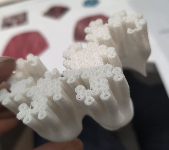
6.1 Dragon’s Feet

Here is an example of turning the dragon curve into a space-filling surface. Each iteration is recorded and offset in depth, all of which inform the generation of a surface that loosely flows through each of them. This was again achieved with Rhino and Grasshopper.
I don’t believe this geometry has a name beyond ‘the developing dragon curve’, so I’ve called it ‘Dragon’s Feet.’
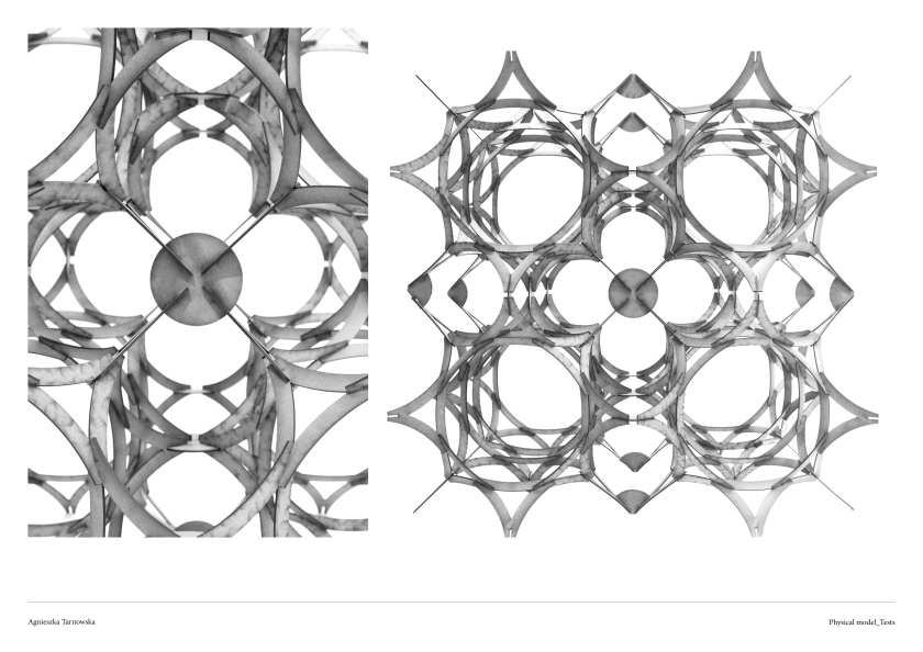
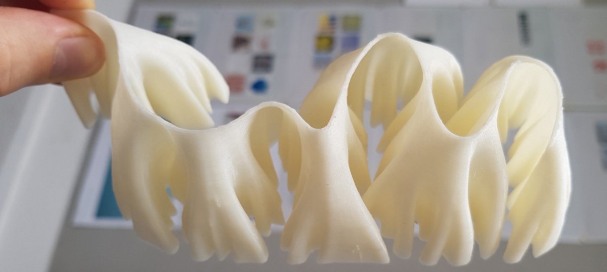
Adding a little thickness to the model allow us to 3D print it.
3d Printed Dragon Curve.jpg
Developing Dragon Curve: Dragon’s Feet – 3D Print

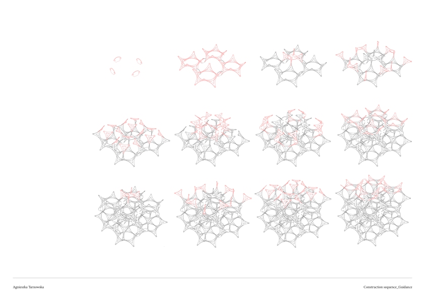
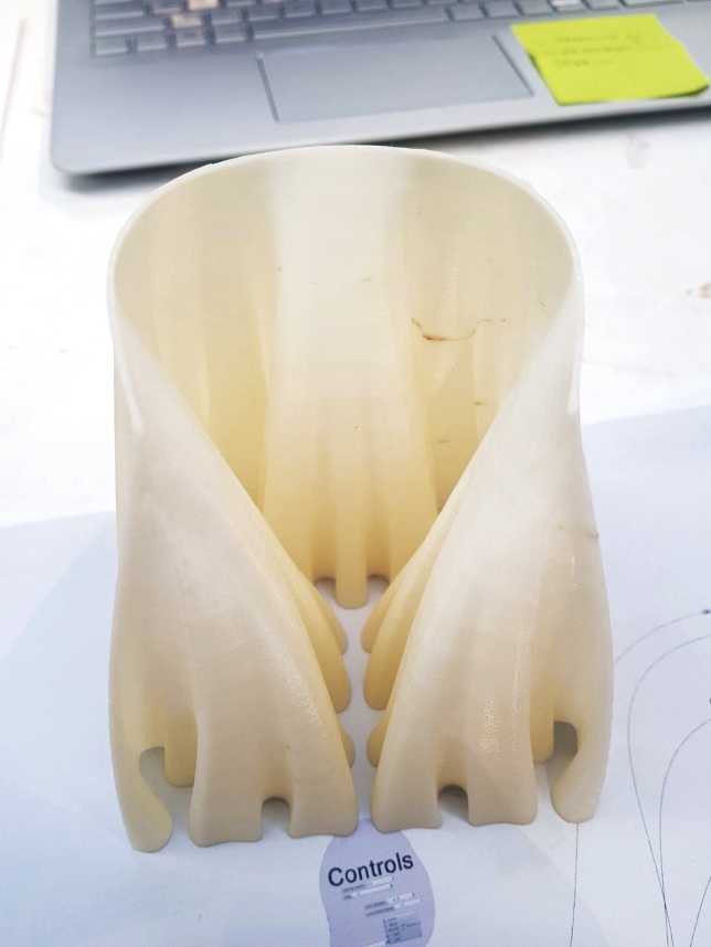
6.2 Hilbert’s Curtain

Here is the Hilbert Curve going through the same process, which I am aptly naming ‘Hilbert’s Curtain.’
3D Printed Developing Hilbert Curve
Developing Hilbert Curve: Hilbert’s Curtain – 3D Print
3D Printing Space-Filling Curves with Henry Segerman at Numberphile:
‘Developing Fractal Curves’ by Geoffrey Irving & Henry Segerman:

6.3 Developing Whale Curve

Unsurprisingly this can also be done with differentially grown curve. The respective difference being that this method fills a specific space in a less controlled manner.
In this case with Kangaroo 2 is used to grow a curve into the shape of a whale. Like before, each iteration is used to inform a single-surface geometry.
Developing-Whale-Curve-b.gif
Iterative Steps of the Differentially Grown Whale Curve

3D print of the different recursive steps of a space-filling curve
Developing Whale Curve – 3D Print

The Wishing Well

something caught in between dimensions – on its way to becoming more.

Summary

The Wishing Well is the physical manifestation, a snap-shot, of a creature caught in between dimensions – frozen in time. It is a digital entity that has been extracted from its home in the fractured planes of the mathematical realm; a differentially grown curve in bloom, organically filling space in the material world.

The notion of geometry in between dimensions is explored in a previous post: Shapes, Fractals, Time & the Dimensions they Belong to


Description

The piece will be built from the bottom-up. Starting with the profile of a differentially grown curve (a squiggly line), an initial layer will be set in pieces of 2 x 4 inch wooden studs (38 x 89 millimeter profile) laid flat, and anchored to the ground. Each subsequent layer will be built upon and fixed to the last, where each new layer is a slightly smoother version than the last. 210 layers will be used to reach a height of 26 feet (8 meters). The horizontal spaces in between each of the pieces will automatically generate hand and foot holes, making the structure easily climbable. The footprint of the build will be bound to a space 32 x 32 feet.

The design may utilize two layers, inner and out, that meet at the top to increase the structural integrity for the whole build. It will be lit from within, either from the ground with spotlights or with LED strip lights following patterns along the walls.

Different Recursive Steps of a Dragon Curve

Ambition

At the Wishing Well, visitors embark on a small journey, exploring the uniquely complex geometry of the structure before them. As they approach the foot of the well, it will stand towering above them, undulating organically across the landscape. The nature of the structure’s curves beckons visitors to explore the piece’s every nook and cranny. Moreover, its stature grants a certain degree of shelter to any traveller seeking refuge from the Playa’s extreme weather conditions. The well’s shape and scale allows natural, and artificial, light to interact in curious ways with the structure throughout the day and night. The horizontal gaps between every ‘brick’ in the wall allows light to filter through each layer, which in turn casts intriguing shadows across the desert. This perforation also allows Burners to easily, and relatively safely, scale the face of the build. Visitors will have the opportunity to grant a wish by writing it down on a tag and fixing it to the well’s interior.

171108 - Burning Man Timber Brick Laying Proposal View 2.jpg


Philosophy

If you had one magical (paradox free) wish, to do anything you like, what would it be?

Anything can be wished for at the Wishing Well, but a wish will not come true if it is deemed too greedy. Visitors must write their wish down on a tag and fix it to the inside of the well. They must choose wisely, as they are only allowed one. Additionally, they may choose to leave a single, precious, offering. However, if the offering does not burn, it will not be accepted. Visitors will also find that they must tread lightly on other people’s wishes and offerings.

The color of the tag and offering are important as they are associated with different meanings:

  • â–º PINK – love
  • â–º RED – happiness, joy, success, good luck, passion, vitality, celebration
  • â–º ORANGE – change, adaptability, spontaneity, concentration
  • â–º YELLOW – nourishment, warmth, clarity, empathy, being free from worldly cares
  • â–º GREEN – growth, balance, healing, self-assurance, benevolence, patience
  • â–º BLUE – conservation, healing, relaxation, exploration, trust, calmness
  • â–º PURPLE – spiritual awareness, physical and mental healing
  • â–º BLACK – profoundness,  stability, knowledge, trust, adaptability, spontaneity,
  • â–º WHITE – mourning, righteousness, purity, confidence, intuition, spirits, courage

The Wishing Well is a physical manifestation of the wishes it holds. They are something caught in between – on their way to becoming more. I wish for guests to reflect on where they’ve been, where they are, where they are going, and where they wish to go.

171108 - Burning Man Timber Brick Laying Proposal View 1.jpg

Shapes, Fractals, Time &, the Dimensions they Belong to

First, second and third dimensions, and why fractals don’t belong to any of them, as well as what happens when you get into higher dimensions.

Foreword

In this post, I’m going to try my best to explain the first, second, and third dimensions, and why fractals don’t belong to any of them, as well as what happens when you get into higher dimensions. But before getting into the nitty-gritty of the subject, I think it’s worth prefacing this post with a short note on the nature of mathematics itself:

Alain Badiou said that mathematics is a rigorous aesthetic; it tells us nothing of real being, but forges a fiction of intelligible consistency. That being said, I think it’s interesting to think about whether or not mathematics were invented or discovered – whether or not numbers exist outside of the human mind.

While I don’t have an answer to this question (and there are at least three different schools of thought on the subject), I do think it’s important to keep in mind that we only use math as a tool to measure and represent ‘real world’ things. In other words, our knowledge of mathematics has its limitations as far as understanding the space-time continuum goes.


1.0 Traditional Dimensions

In physics and mathematics, dimensions are used to define the Cartesian plains. The measure of a mathematical space is based on the number of variables require to define it. The dimension of an object is defined by how many coordinates are required to specify a point on it.

It’s important to note that there is no ‘first’ or ‘second’ dimension. It’s a bit like pouring three cups of water into a vase and asking someone which cup is the first one. The question doesn’t even make sense.

Capture4
Excerpt from ‘minutephysics’
We usually arbitrarily pick a dimension and calling it the ‘first’ one.


1.1 – Zero Dimensions

 O2FFp

Something of zero dimensions give us a point. While a point can inhabit (and be defined in) higher dimensions, the point itself has a dimension of zero; you cannot move anywhere on a point.

1.2 – One Dimension

R1

A line or a curve gives us a one-dimensional object, and is typically bound by two zero-dimensional things.
Only one coordinate is required to define a point on the curve.
Similarly to the point, a curve can inhabit higher dimension (i.e. you can plot a curve in three dimensions), but as an object, it only possesses one dimension.
Another way to think about it is: if you were to walk along this curve, you could only go forwards or backward – you’d only have access to one dimension, even though you’d be technically moving through three dimensions.


1.3 – Two Dimensions

 R2

Surfaces or plains gives us two-dimensional shapes, and are typically bound by one-dimensional shapes (lines/curves).

A plain can be defined by x&y, y&z or x&z; more complex surfaces are commonly defined by u&v values. These variable are arbitrary, what is important is that there are two of them.

A surface can live in three+ dimensions, but still only possesses two dimension. Two coordinate are required to define a point on a surface. For example a sphere is a three-dimensional object, but the surface of a sphere is two-dimensional – a point can be defined on the surface of a sphere with latitude and longitude.


1.4 – Three Dimensions

rotated-cube

A volume gives us a three-dimensional shape, and can be bound by two-dimensional shapes (surfaces).

Shapes in three dimensions are most commonly represented in relation to an x, y and z axis. If a person were to swim in a body of water, their position could be defined by no less than three coordinates – their latitude, longitude and depth. Traveling through this body of water grants access to three dimensions.


2.0 Fractal Dimensions

Fractals can be generally classified as shapes with a non-integer dimension (a dimension that is not a whole number). They may or may not be self-similar, but are typically measured by their properties at different scales.

Felix Hausdorff and Abram Besicovitch demonstrated that, though a line has a dimension of one and a square a dimension of two, many curves fit in-between dimensions due to the varying amounts of information they contain. These dimensions between whole numbers are known as Hausdorff-Besicovitch dimensions.


2.1 – Between the First & Second Dimensions

A line or a curve gives us a one-dimensional object that allows us to move forwards and backwards, where only one coordinate is required to define a point on them.

Surfaces give us two-dimensional shapes, where two coordinate are required to define a point on them.

ch08_04-660x313
Here is a shape that cannot be classified as a one-dimensional shape, or a two-dimensional shape. It can be plotted in two dimensions, or even three dimensions, but the object itself does not have access the two whole dimensions.

If you were to walk along the shape starting from the base, you could go forwards and backwards, but suddenly you have an option that’s more than forwards and backwards, but less than left and right.

You cannot define a point on this shape with a single coordinate, and a two coordinate system would define a point off of the shape more often than not.

hausdorff_dimension_by_dnangel7
Each fractal has a unique dimensional measure based on how much space they fill.


2.2 – Between the Second & Third Dimensions

koch-render.png
Developing Koch Snowflake
The same logic applies when exploring fractals plotted in three dimensions:

Surfaces give us two-dimensional shapes, where two coordinate are required to define a point on them.

A volume gives us a three-dimensional shape where a point could be defined by no less than three coordinates.

While these models live in three dimensions, they do not quite have access to all of them. You cannot define a point on them with two coordinates: they are more than a surface and less than a volume.

d60e89184e7eb476ccfce4112c948f47
Fourth Iteration Menger Sponge
The Menger Sponge for example has (mathematically) a volume of zero, but an infinite surface area.


2.3 – Calculating Fractal Dimensions

The following are three methods of calculating Hausdorff-Besicovitch dimension:
• The exactly self-similar method for calculating dimensions of mathematically generated repeating patterns.
• The Richardson method for calculating a dimensional slope.
• The box-counting method for determining the ratios of a fractal’s area or volume.


On another note:

In theory, higher (non-integer) dimensional fractals are possible.
As far as I’m concerned however, they’re not particularly good for anything in a three-dimensional world. You are more than welcome to prove me wrong though.


3.0 Higher Dimensions

Sadly, living in a three-dimensional world makes it especially difficult to think about, and nearly impossible to visualise, higher dimensions. This is in the same way that a two-dimensional being would find it impossibly hard to think about our three-dimensional world, a subject explored in the novel ‘Flatland’ by Edwin A. Abbott.

That being said, it’s plausible that we experience much higher dimensions that are just too hard to perceive. For example, an ant walking along the surface of a sphere will only ever perceive two dimensions, but is moving through three dimensions, and is subject to the fourth (temporal) dimension.


3.1 – The Fourth Dimension (Temporal)

If we consider time an additional variable, then despite the fact that we live in a three dimensional world, we are always subject to (even if we cannot visualize) a fourth dimension.

Neil deGrasse Tyson puts it quite plainly by saying:
“[…] you have never met someone at a place, unless it was at a time; you have never met someone at a time, unless it was at a place […]”

Suppose we call our first three dimensions x, y & z, and our fourth t: latitude, longitude, altitude and time, respectively. In this instance, time is linear, and time & space are one. As if the universe is a kind of film, where going forwards and backwards in time will always yield the exact same outcome; no matter how many times you return to a point in point time, you will always find yourself (and everything else) in the exact same place.
However time is only linear for us as three-dimensional beings. For a four-dimensional being, time is something that can be moved through as freely as swimming or walking.
Capture
Excerpt from ‘Seeker’


3.2 – The Fourth Dimension (Spacial)

If we explore spacial dimensions, a four-dimensional object may be achieved by ‘folding’ three-dimensional objects together. They cannot exist in our three-dimensional world, but there are tricks to visualise them.

roj5

We know that we can construct a cube by folding a series of two-dimensional surfaces together, but this is only possible with the third dimension, which we have access to.

Cube-Rotation


If we visualise, in two dimensions, a cube rotating (as seen above), it looks like each surface is distorting, growing and shrinking, and is passing through the other. However we are familiar enough with the cube as a shape to know that this is simply a trick of perspective – that objects only look smaller when they are farther away.

In the same way that a cube is made of six squares, a four-dimensional cube (hypercube or tesseract), is made of eight cubes.

  • A line is bound by two zero-dimensional things
  • A square is bound by four one-dimensional shapes
  • A cube is bound by six two-dimensional surfaces
  • A hypercube, bound by eight three-dimensional volumes

It looks like each cube is distorting, growing and shrinking, and passing through the other. This is because we can only represent eight cubes folding together in the fourth dimension with three-dimensional perspective animation.

HCube-Folding
3D representation of eight cubes folding in 4D space to form a Hypercube

Perspective makes it look like the cubes are growing and shrinking, when they are simply getting closer and further in four-dimensional space. If somehow we could access this higher dimension, we would see these cubes fold together unharmed the same way forming a cube leaves each square unharmed.

Below is a three-dimensional perspective view of hypercube rotating in four dimensions, where (in four-dimensional space) all eight cubes are always the same, but are being subjected to perspective.


AK986lrhNHiZq


3.3 – The Fifth and Sixth Dimensions

On the temporal side of things, adding the ability to move ‘left & right’ and ‘up & down’ in time gives us the fifth and sixth dimensions.

(For example: x, y, z, t1, t2, t3)

This is a space where one can move through time based on probability and permutations of what could have been, is, was, or will be on alternate timelines. For any one point in this space, there are six coordinates that describe its position.

terminator-arnold-as-terminator__131206182643
In spacial dimensions, it is theoretically possible to fold four-dimensional objects with a fifth dimension. However, it becomes increasingly difficult for us to visualise what is happening to the shapes that we’re folding.
s1-coxeter
In theory, objects can keep being folded together into higher and higher spacial dimensions indefinitely. (R1, R2, R3,R4,R5, R6, R7 etc.)

There’s a terrific explanation of what happens to platonic solids and regular polytopes in higher dimensions on Numberphile: https://youtu.be/2s4TqVAbfz4


3.4 – Even Higher Dimensions

If we can take a point and move it through space and time, including all the futures and pasts possible, for that point, we can then move along a number line where the laws of gravity are different, the speed of light has changed.

Dimensions seven though ten are different universes with different possibilities, and impossibilities, and even different laws of physics. These grasp all the possibilities and permutations of how each universe operates, and the whole of reality with all the permutations they’re in, throughout all of time and space. The highest dimension is the encompassment of all of those universes, possibilities, choices, times, places all into a single ‘thing.’

These ten time-space dimensions belong to something called Super-string Theory, which is what physicists are using to help us understand how the universe works.

Calabi_yau_formatted.svg
Cross section of the quintic Calabi–Yau manifold
There may very well be a link between temporal dimensions and spacial dimensions. For all I know, they are actually the same thing, but thinking about it for too long makes my head hurt. If the topic interests you, there is a philosophical approach to the nature of time called ‘eternalism’, where one may find answers to these questions. Other dimensional models include M-Theory, which suggests there are eleven dimensions.

While we don’t have experimental or observational evidence to confirm whether or not any of these additional dimensions really exist, theoretical physicists continue to use these studies to help us learn more about how the universe works. Like how gravity affects time, or the higher dimensions affect quantum theory.

TriNect

The aim is to generate an architectural response through a playful loop between the digital and the physical. Digital tools such as Rhino and Grasshopper are used  in order to carry out analysis and generate buildable three-dimensional forms. Interplay between physical fabrication and digital experiments enable to become an inventor of a system. Here is mine.

TriNect is a flexible system of triangular elements with slots at their vertices. Elements interlock with one another creating different space filling polyhedra. The system can be applied in various scales and adapted for different needs.

TriNect

TriNect1TriNect2TriNect3TriNect4TriNect5TriNect6TriNect7TriNect8TriNect9TriNect10TriNect11TriNect12TriNect13TriNect14TriNect15TriNect16TriNect17TriNect18TriNect19TriNect20TriNect21TriNect22TriNect23TriNect24TriNect25TriNect26TriNect27TriNect28TriNect29TriNect30TriNect31TriNect32TriNect33TriNect34TriNect35TriNect36TriNect37TriNect38TriNect39TriNect40TriNect41TriNect42TriNect43TriNect44TriNect45TriNect46TriNect47TriNect48TriNect49TriNect50TriNect51