Foreword
This post is the third installment of sort of trilogy, after Shapes, Fractals, Time & the Dimensions they Belong to, and Developing Space-Filling Fractals. While it’s not important to have read either of those posts to follow this one, I do think it adds a certain level of depth and continuity.
Regarding my previous entries, it can be difficult to see how any of this has to do with architecture. In fact I know a few people who think studying fractals is pointless.
Admittedly I often struggle to explain to people what fractals are, let alone how they can influence the way buildings look. However, I believe that this post really sheds light on how these kinds of studies may directly influence and enhance our understanding (and perhaps even the future) of our built environment.
On a separate note, I heard that a member of the architectural academia said “forget biomimicry, it doesn’t work.”
Firstly, I’m pretty sure Frei Otto would be rolling over in his grave.
Secondly, if someone thinks that biomimicry is useless, it’s because they don’t really understand what biomimicry is. And I think the same can be said regarding the study of fractals. They are closely related fields of study, and I wholeheartedly believe they are fertile grounds for architectural marvels to come.
7.0 Introduction to Shells
As far as classification goes, shells generally fall under the category of two-dimensional shapes. They are defined by a curved surface, where the material is thin in the direction perpendicular to the surface. However, assigning a dimension to certain shells can be tricky, since it kinda depends on how zoomed in you are.
A strainer is a good example of this – a two-dimensional gridshell. But if you zoom in, it is comprised of a series of woven, one-dimensional wires. And if you zoom in even further, you see that each wire is of course comprised of a certain volume of metal.
This is a property shared with many fractals, where their dimension can appear different depending on the level of magnification. And while there’s an infinite variety of possible shells, they are (for the most part) categorizable.
7.1 – Single Curved Surfaces
Analytic geometry is created in relation to Cartesian planes, using mathematical equations and a coordinate systems. Synthetic geometry is essentially free-form geometry (that isn’t defined by coordinates or equations), with the use of a variety of curves called splines. The following shapes were created via Synthetic geometry, where we’re calling our splines ‘u’ and ‘v.’
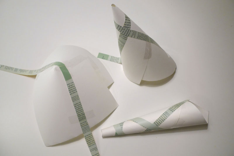
These curves highlight each dimension of the two-dimensional surface. In this case only one of the two ‘curves’ is actually curved, making this shape developable. This means that if, for example, it was made of paper, you could flatten it completely.
Uniclastic: Conoid (Conical paraboloid)
In this case, one of them grows in length, but the other still remains straight. Since one of the dimensions remains straight, it’s still a single curved surface – capable of being flattened without changing the area. Singly curved surfaced may also be referred to as uniclastic or monoclastic.
7.2 – Double Curved Surfaces
These can be classified as synclastic or anticlastic, and are non-developable surfaces. If made of paper, you could not flatten them without tearing, folding or crumpling them.
In this case, both curves happen to be identical, but what’s important is that both dimensions are curving in the same direction. In this orientation, the dome is also under compression everywhere.
The surface of the earth is double curved, synclastic – non-developable. “The surface of a sphere cannot be represented on a plane without distortion,” a topic explored by Michael Stevens: https://www.youtube.com/watch?v=2lR7s1Y6Zig
7.3 – Translation vs Revolution
This shape was achieved by sweeping a straight line over a straight path at one end, and another straight path at the other. This will work as long as both rails are not parallel. Although I find this shape perplexing; it’s double curvature that you can create with straight lines, yet non-developable, and I can’t explain it..
The hyperboloid has been a popular design choice for (especially nuclear cooling) towers. It has excellent tensile and compressive properties, and can be built with straight members. This makes it relatively cheap and easy to fabricate relative to it’s size and performance.
8.0 Geodesic Curves
These are singly curved curves, although that does sound confusing. A simple way to understand what geodesic curves are, is to give them a width. As previously explored, we know that curves can inhabit, and fill, two-dimensional space. However, you can’t really observe the twists and turns of a shape that has no thickness.
A ribbon is essentially a straight line with thickness, and when used to follow the curvature of a surface (as seen above), the result is a plank line. The term ‘plank line’ can be defined as a line with an given width (like a plank of wood) that passes over a surface and does not curve in the tangential plane, and whose width is always tangential to the surface.
Since one-dimensional curves do have an orientation in digital modeling, geodesic curves can be described as the one-dimensional counterpart to plank lines, and can benefit from the same definition.
The University of Southern California published a paper exploring the topic further: http://papers.cumincad.org/data/works/att/f197.content.pdf
8.1 – Basic Grid Setup
For simplicity, here’s a basic grid set up on a flat plane:
We start by defining two points anywhere along the edge of the surface. Then we find the geodesic curve that joins the pair. Of course it’s trivial in this case, since we’re dealing with a flat surface, but bear with me.
We can keep adding pairs of points along the edge. In this case they’re kept evenly spaced and uncrossing for the sake of a cleaner grid.
After that, it’s simply a matter of playing with density, as well as adding an additional set of antagonistic curves. For practicality, each set share the same set of base points.
He’s an example of a grid where each set has their own set of anchors. While this does show the flexibility of a grid, I think it’s far more advantageous for them to share the same base points.
8.2 – Basic Gridshells
The same principle is then applied to a series of surfaces with varied types of curvature.
First comes the shell (a barrel vault in this case), then comes the grid. The symmetrical nature of this surface translates to a pretty regular (and also symmetrical) gridshell. The use of geodesic curves means that these gridshells can be fabricated using completely straight material, that only necessitate single curvature.
The same grid used on a conical surface starts to reveal gradual shifts in the geometry’s spacing. The curves always search for the path of least resistance in terms of bending.
This case illustrates the nature of geodesic curves quite well. The dome was free-formed with a relatively high degree of curvature. A small change in the location of each anchor point translates to a large change in curvature between them. Each curve looks for the shortest path between each pair (without leaving the surface), but only has access to single curvature.
Structurally speaking, things get much more interesting with anticlastic curvature. As previously stated, each member will behave differently based on their relative curvature and orientation in relation to the surface. Depending on their location on a gridshell, plank lines can act partly in compression and partly in tension.
On another note:
While geodesic curves make it far more practical to fabricate shells, they are not a strict requirement. Using non-geodesic curves just means more time, money, and effort must go into the fabrication of each component. Furthermore, there’s no reason why you can’t use alternate grid patterns. In fact, you could use any pattern under the sun – any motif your heart desires (even tessellated puppies.)
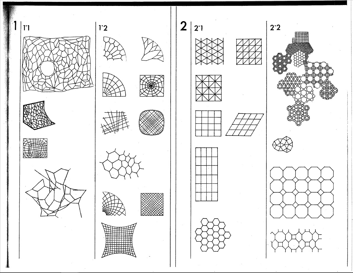
Here are just a few of the endless possible pattern. They all have their advantages and disadvantages in terms of fabrication, as well as structural potential.
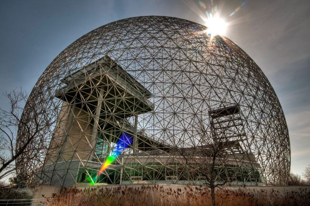
Gridshells with large amounts of triangulation, such as Buckminster Fuller’s geodesic spheres, typically perform incredibly well structurally. These structure are also highly efficient to manufacture, as their geometry is extremely repetitive.
Gridshells with highly irregular geometry are far more challenging to fabricate. In this case, each and every piece had to be custom made to shape; I imagine it must have costed a lot of money, and been a logistical nightmare. Although it is an exceptionally stunning piece of architecture (and a magnificent feat of engineering.)
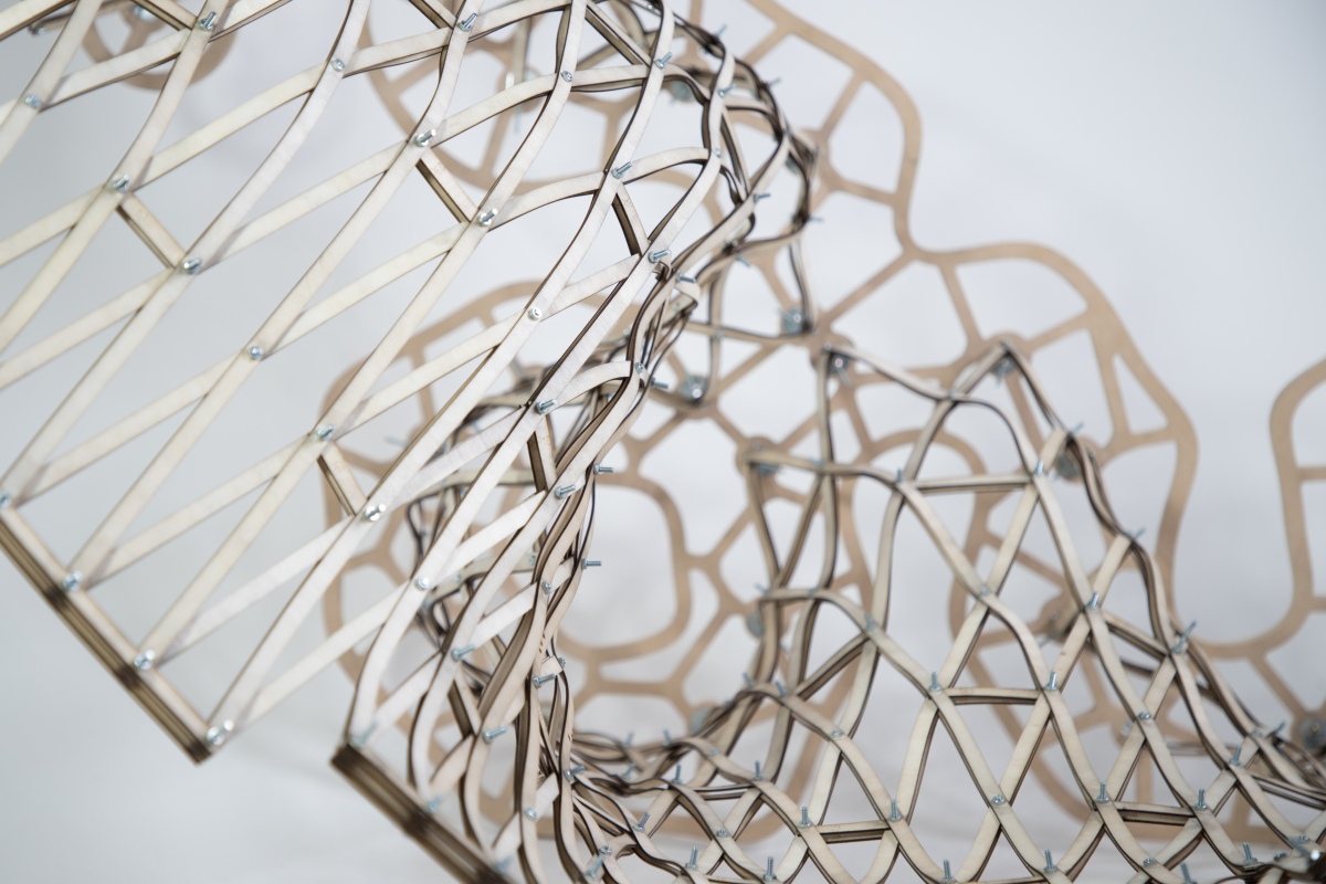
8.3 – Gridshell Construction
In our case, building these shells is simply a matter of converting the geodesic curves into planks lines.
The whole point of using them in the first place is so that we can make them out of straight material that don’t necessitate double curvature. This example is rotating so the shape is easier to understand. It’s grid is also rotating to demonstrate the ease at which you can play with the geometry.
This is what you get by taking those plank lines and laying them flat. In this case both sets are the same because the shell happens to the identicall when flipped. Being able to use straight material means far less labour and waste, which translates to faster, and or cheaper, fabrication.
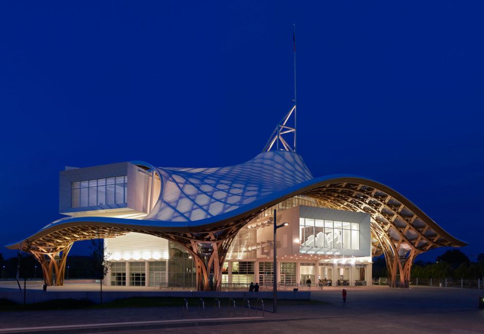
An especially crucial aspect of gridshells is the bracing. Without support in the form of tension ties, cable ties, ring beams, anchors etc., many of these shells can lay flat. This in and of itself is pretty interesting and does lends itself to unique construction challenges and opportunities. This isn’t always the case though, since sometimes it’s the geometry of the joints holding the shape together (like the geodesic spheres.) Sometimes the member are pre-bent (like Pompidou-Metz.) Although pre-bending the timber kinda strikes me as cheating thought.. As if it’s not a genuine, bona fide gridshell.
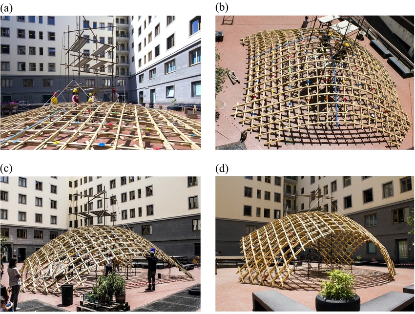
This is one of the original build method, where the gridshell is assembled flat, lifted into shape, then locked into place.
9.0 Form Finding
Having studied the basics makes exploring increasingly elaborate geometry more intuitive. In principal, most of the shells we’ve looked are known to perform well structurally, but there are strategies we can use to focus specifically on performance optimization.
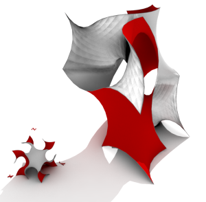
9.0 – Minimal Surfaces
These are surfaces that are locally area-minimizing – surfaces that have the smallest possible area for a defined boundary. They necessarily have zero mean curvature, i.e. the sum of the principal curvatures at each point is zero. Soap bubbles are a great example of this phenomenon.
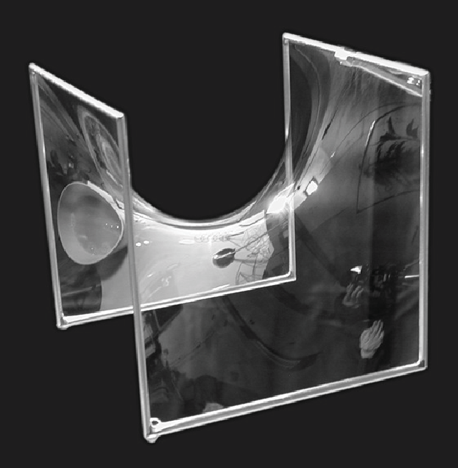
Hyperbolic Paraboloid Soap Bubble [Source: Serfio Musmeci’s “Froms With No Name” and “Anti-Polyhedrons”]Soap film inherently forms shapes with the least amount of area needed to occupy space – that minimize the amount of material needed to create an enclosure. Surface tension has physical properties that naturally relax the surface’s curvature.
We can simulate surface tension by using a network of curves derived from a given shape. Applying varies material properties to the mesh results in a shape that can behaves like stretchy fabric or soap. Reducing the rest length of each of these curves (while keeping the edges anchored) makes them pull on all of their neighbours, resulting in a locally minimal surface.
Here are a few more examples of minimal surfaces you can generate using different frames (although I’d like stress that the possibilities are extremely infinite.) The first and last iterations may or may not count, depending on which of the many definitions of minimal surfaces you use, since they deal with pressure. You can read about it in much greater detail here: https://tinyurl.com/ya4jfqb2
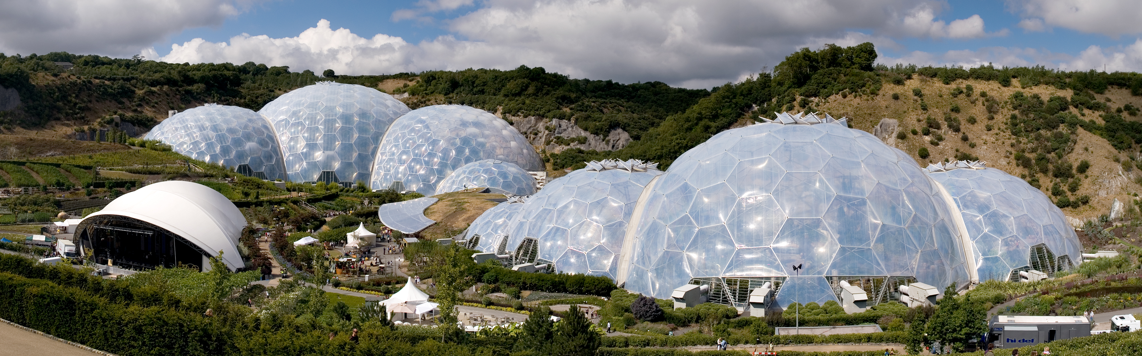
Here we have one of the most popular examples of minimal surface geometry in architecture. The shapes of these domes were derived from a series of studies using clustered soap bubbles. The result is a series of enormous shells built with an impressively small amount of material.
Triply periodic minimal surfaces are also a pretty cool thing (surfaces that have a crystalline structure – that tessellate in three dimensions):
9.2 – Catenary Structures
Another powerful method of form finding has been to let gravity dictate the shapes of structures. In physics and geometry, catenary (derived from the Latin word for chain) curves are found by letting a chain, rope or cable, that has been anchored at both end, hang under its own weight. They look similar to parabolic curves, but perform differently.
A net shown here in magenta has been anchored by the corners, then draped under simulated gravity. This creates a network of hanging curves that, when converted into a surface, and mirrored, ultimately forms a catenary shell. This geometry can be used to generate a gridshell that performs exceptionally well under compression, as long as the edges are reinforced and the corners are braced.
While I would be remiss to not mention Antoni Gaudí on the subject of catenary structure, his work doesn’t particularly fall under the category of gridshells. Instead I will proceed to gawk over some of the stunning work by Frei Otto.
Of course his work explored a great deal more than just catenary structures, but he is revered for his beautiful work on gridshells. He, along with the Institute for Lightweight Structures, have truly been pioneers on the front of theoretical structural engineering.
9.3 – Biomimicry in Architecture
Frei Otto is a fine example of ecological literacy at its finest. A profound curiosity of the natural world greatly informed his understanding of structural technology. This was all nourished by countless inquisitive and playful investigations into the realm of physics and biology. He even wrote a series of books on the way that the morphology of bird skulls and spiderwebs could be applied to architecture called Biology and Building. His ‘IL‘ series also highlights a deep admiration of the natural world.
Of course he’s the not the only architect renown their fascination of the universe and its secrets; Buckminster Fuller and Antoni Gaudí were also strong proponents of biomimicry, although they probably didn’t use the term (nor is the term important.)
Gaudí’s studies of nature translated into his use of ruled geometrical forms such as hyperbolic paraboloids, hyperboloids, helicoids etc. He suggested that there is no better structure than the trunk of a tree, or a human skeleton. Forms in biology tend to be both exceedingly practical and exceptionally beautiful, and Gaudí spent much of his life discovering how to adapt the language of nature to the structural forms of architecture.
Fractals were also an undisputed recurring theme in his work. This is especially apparent in his most renown piece of work, the Sagrada Familia. The varying complexity of geometry, as well as the particular richness of detail, at different scales is a property uniquely shared with fractal nature.
Antoni Gaudí and his legacy are unquestionably one of a kind, but I don’t think this is a coincidence. I believe the reality is that it is exceptionally difficult to peruse biomimicry, and especially fractal geometry, in a meaningful way in relation to architecture. For this reason there is an abundance of superficial appropriation of organic, and mathematical, structures without a fundamental understanding of their function. At its very worst, an architect’s approach comes down to: ‘I’ll say I got the structure from an animal. Everyone will buy one because of the romance of it.”
That being said, modern day engineers and architects continue to push this envelope, granted with varying levels of success. Although I believe that there is a certain level of inevitability when it comes to how architecture is influenced by natural forms. It has been said that, the more efficient structures and systems become, the more they resemble ones found in nature.
Euclid, the father of geometry, believed that nature itself was the physical manifestation of mathematical law. While this may seems like quite a striking statement, what is significant about it is the relationship between mathematics and the natural world. I like to think that this statement speaks less about the nature of the world and more about the nature of mathematics – that math is our way of expressing how the universe operates, or at least our attempt to do so. After all, Carl Sagan famously suggested that, in the event of extra terrestrial contact, we might use various universal principles and facts of mathematics and science to communicate.